Excel is all about working with numbers. However, if your data consists of too much text, you don’t have to worry at all. Excel provides several functions that make it easier to manipulate text strings. These functions let you easily find a string, count the characters in a string, remove extra spaces from a string, join two or more strings, and perform other similar tasks on the textual data.
What are Text functions in Excel?
Text Functions are Microsoft Excel’s native functions that allow transforming or analyzing textual data. Excel provides a total of 30+ Text functions and many of these are often used by people for data analysis. This post highlights 10 such Text functions, with their uses and examples.
10 Text Functions in Excel with Examples
Following is the list of top 10 functions in Excel:
- FIND
- LEN
- LEFT
- RIGHT
- MID
- SUBSTITUTE
- UPPER
- TRIM
- CONCATENATE
- TEXT
Let’s take a detailed look at these functions, one by one.
1] FIND
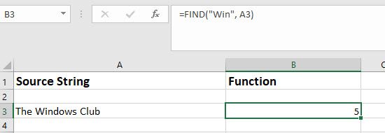
The FIND function allows you to find a text string within another. It returns the position at which a character or string begins within another text string.
Syntax
FIND(find_text, within_text, [start_num])
- find_text argument is used to enter the text the user wants to search.
- within-text argument takes the text which contains the text that needs to be found.
- [start_num] is an optional argument that takes the position from where to start the search. It takes the value 1 by default.
Example
Let us say the A3 cell in an Excel sheet contains the string ‘The Windows Club’. If the user wants to find the position of ‘Win’ within the string, he may use the ‘Find’ functions as:
f(x)=FIND("Win", A1)
The output of the above function will be 5, as 5 represents the starting position of the text ‘Win’ within ‘The Windows Club’.
Note: The FIND function is case-sensitive. If you do not want to match the case, you can use the SEARCH function, which has the same syntax as the FIND function.
Read: How to use the new TEXTSPLIT function in Excel
2] LEN
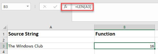
The LEN function calculates the length of the string, i.e. the number of characters present in a string. It counts the spaces as characters.
Syntax
LEN(text)
- text argument takes the string whose length the user wants to find.
Example
In the above example, if the user wants to find the length of the string ‘The Windows Club’, he may use the ‘LEN’ function as:
f(x)=LEN (A3)
The output of the above function will be 16, as there are 16 characters in the string ‘The Windows Club’, including spaces.
Also read: Arrows keys are not working in Microsoft Excel.
3] LEFT
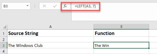
The LEFT function returns several successive characters from the left side of a string, based on the number specified by the user.
Syntax
LEFT(text, [num_chars])
- text argument is used to specify the string that contains the characters that need to be found.
- [num_chars] specifies the number of characters to be extracted from the left of the main string. This argument is optional. It takes ‘1’ as a default value, if not specified by the user.
Example
In the same example as stated above, if the user wants to extract the first 7 characters from ‘The Windows Club’, he may use the ‘LEFT’ function as:
f(x)=LEFT (A3, 7)
The output of the above function will be The Win, as these are the 7 leftmost characters in the string ‘The Windows Club’, including spaces.
4] RIGHT
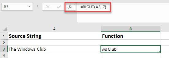
The RIGHT function is used to extract several characters from the extreme right of a string.
Syntax
RIGHT(text, [num_chars])
- text argument specifies the string that contains the desired characters.
- [num_chars] argument specifies the number of characters that need to be extracted, moving from the extreme right to the left of the string. This is an optional argument that takes ‘1’ as the default value if left unspecified.
Example
Taking the same example, if the user wants to extract the last 7 characters from the string ‘The Windows Club’, he may use the ‘RIGHT’ function as:
f(x)=RIGHT(A3, 7)
The output of the above function will be ws Club, since they are the 7 rightmost characters in ‘The Windows Club’, including spaces.
5] MID
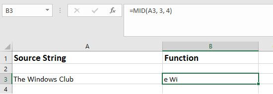
The MID function returns several consecutive characters or a substring from the middle of another string.
Syntax
MID(text, start_num, num_chars)
- text argument takes the string that contains the desired characters.
- start_num argument takes the position from where to start extracting the characters.
- num_chars argument takes the number of characters the user wants to extract from the string.
Example
In the above example, if the user wants to extract 4 characters starting from the 3rd character in the string ‘The Windows Club’, he may use the ‘MID’ function as:
f(x)=MID(A3, 3, 4)
The output of the above function will be e Wi, as ‘e’ is the third character and staring from ‘e’ counting spaces as well, ‘e Wi’ are the 4 consecutive characters in the string ‘The Windows Club’.
6] SUBSTITUTE
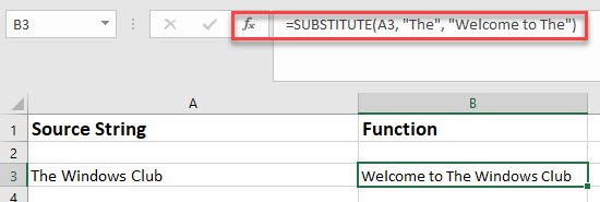
The Substitute function replaces an existing text with a new text in a given string.
Syntax
SUBSTITUTE(text, old_text, new_text, [instance_num])
- text argument specifies the main string.
- old_text argument specifies the text that needs to be replaced.
- new_text argument specifies the text that needs to be put in place of the existing text.
- [instance_num] argument specifies which instance (or occurrence) of the existing text is to be replaced. This is an optional argument. If you specify this value, only that instance of the text will be replaced; otherwise, all the instances of the existing text will be replaced with the new text.
Example
In the same example, if the user wants to substitute ‘Welcome to The’ for ‘The’ in ‘The Windows Club’, he may use the ‘SUBSTITUTE’ function as:
f(x)=SUBSTITUTE(A3, "The", "Welcome to The")
The output of the above function will be Welcome to The Windows Club, as the substitute function has replaced ‘The’ with ‘Welcome to The’ in the text string ‘The Windows Club’.
7] UPPER
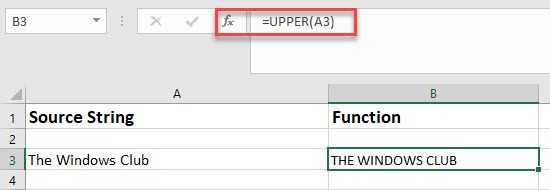
The UPPER function converts a string into uppercase, i.e., it returns a string after capitalizing each letter.
Syntax
UPPER(text)
- text argument takes the string that needs to be capitalized.
Example
Following the same example, if the user wants to capitalize each letter in the string ‘The Windows Club’, he may use the ‘UPPER’ function as:
f(x)=UPPER(A3)
The output of the above function will be THE WINDOWS CLUB.
Note:
- If you want to convert a string into lowercase, you may use the LOWER function, having the same syntax as that of the UPPER function.
- If you want to capitalize the first letter of each word in a string, you may use the PROPER function with the same syntax.
8] TRIM
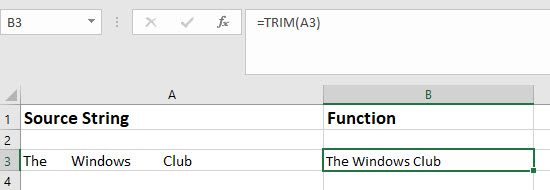
The TRIM function removes all the extra spaces within a string, leaving just 1 space between two words.
Syntax
TRIM(text)
- text argument takes the string with irregular spacing.
Example
In the example stated above, if the user wants to remove unnecessary spaces from the string ‘The Windows Club’, he may use the ‘TRIM’ function as:
f(x)=TRIM(A3)
The output of the above function will be The Windows Club, leaving just a single space between words.
9] CONCATENATE
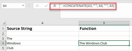
The CONCATENATE function joins two or more strings in Excel.
Syntax
CONCATENATE(text1, [text2], ...)
- text1 argument is mandatory. It takes the first string to join.
- text2 argument takes the additional string to join. You may join up to 255 strings.
Example
Let us say the A3 cell in an Excel sheet contains the string ‘The’, the A4 cell contains the string ‘Windows’, and the A5 cell contains the string ‘Club’. If the user wants to join these strings, he may use the ‘CONCATENATE’ functions as:
f(x)=CONCATENATE(A3, " ", A4, " ", A5)
The output of the above function will be The Windows Club, joining the strings in A3, A4, and A5 cells with spaces between these strings.
Tip: Use the ampersand (&) symbol to concatenate two text strings.
10] TEXT

The TEXT function converts the format of a number from ‘numeric’ to ‘text’. The function can be used to place formatted numbers between text.
Syntax
TEXT(value, format_text)
- value argument takes the numerical value that needs to be formatted.
- format_text argument takes the format that needs to be applied to the value.
Example
Let us say the A2 cell in Excel contains the string ‘The Windows Club started on’ and the A3 cell contains the numeric data ’20-04-2009′; the two of these can be combined in a single sentence using the ‘CONCATENATE’ and the ‘TEXT’ functions as:
f(x)=A2&" "&TEXT(A3,"mmmm d, yyyy")&"."
The output of the above functions will be The Windows Club started on April 20, 2009.
Also read: How to convert currencies in Excel.
What is an example of a text function?
The TEXT function in Excel is used to join a formatted number with a text string. For example, if an Excel sheet contains the string ‘Retails sales surge by’ in cell A1, and the number ‘20000’ in cell A2, then TEXT function can be used to join the content of these two cells as:
f(x)=A1&" "&TEXT(A3,"$ ##,###")&".".
The above function will return ‘Retails sales surge by $20,000.’, where the number 20000 has been formatted using a currency symbol and comma separator.
What is the use of lower function?
The LOWER function is used to change the case of a string to lowercase. If a given string is in uppercase, proper case, or sentence case, the LOWER function will return the string with each of its alphabet converted in small letters. The syntax for LOWER function is LOWER(text), where text specifies the string or reference to the cell that contains the string that needs to be converted into lowercase.
Read Next: Top 15 Financial functions in Microsoft Excel.
Leave a Reply