We know that we can set filters on columns and filter the data with just a click in Microsoft Excel. It can be done by clicking on the ‘Filter’ under the “Data” tab. Apart from just filtering the data based on columns, we can even filter the data set completely based on some conditions. Suppose we want to filter the data set matching the specific criteria, then it can be done using Advance Filter. In this article, I will explain how to use Advance Filter in Excel.
How to use Advance Filter in Excel
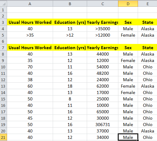
Let me explain this with the sample data of Employees. I have the data set containing Usual Hours Worked, Education in Years, Yearly Earnings, Sex and State. Now, I want to filter the data meeting the conditions as follows,
Condition for Male:
- Usual Hours Worked: 40
- Education: 13
- Yearly Earnings: Greater than 35000
- Gender: Male
- State: Alaska
Condition for Female:
- Usual Hours Worked: Greater than 35
- Education: Greater than 12
- Yearly Earnings: Greater than 12000
- Gender: Female
- State: Alaska
If we see the conditions, we need to filter the data of Male and Female employees separately. I mean, there was an OR condition, and within that, there was AND condition to be met.
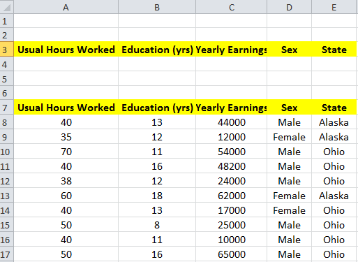
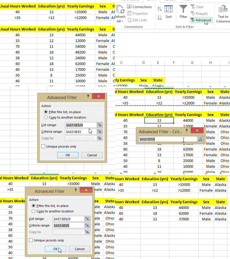
We need to deal with the Excel sheet differently to filter out the data meeting these conditions. This is where advanced filter in Excel comes into the picture. Now, we will prepare the criteria in the same Excel sheet itself. Create two rows above the original data set with the same column names as the already present data as shown below from A3 to E5.
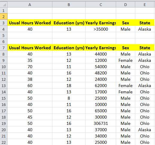
Now, we will fill the criteria columns with the data as mentioned in the conditions. As mentioned in Condition for Male, fill the entire row with the specified columns. So, Row 4 will be filled as shown below.
Repeat the same for the next Row 5 based on Condition for Female as shown below. Now, to clarify, if data in each row are linked with OR condition and data within that row (column-wise data) are linked with AND condition. So, we just created the rows meeting the criteria with which we need to filter the data.
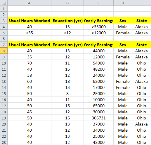
Now, it is time to use the advanced filter in Excel to filter the data. First, click any cell on your original dataset, click the “Data” tab, and click the “Advanced” button. It will automatically fill the List Range. Click on the small button beside the Criteria range. Now, select the criteria range, i.e., A3 to E5, and click on the same small button to set the standards range. Now, click “Ok.” It will filter the data as you want to meet the criteria.
Note: To get this to work, the Column Names of the criteria range should be precisely the same as the column names of the data set.
Advance Filter in Excel allows us to filter the data, meeting the complex queries. So, what query or condition have you used to filter the data? Please let us know through comments if you have anything to add.
Read: How to change the default Numbered List in Word.
How do I use advanced filter unique records only in Excel?
Under the Data tab, select the Advanced Filter, and then ensure the filter is set to Unique records only. It will ensure the discard of any duplicate records. It can also be used when copying data to another cell or applying it at the exact location.
Read: Add Windows Calculator to Excel Quick Access Toolbar
Which action must you take before using the filter feature?
Ensure there is no blank row between the set of data. Otherwise, it will skip the rest of the rows. When setting up the filter, the first row is taken as the header, and the rest of the rows under it are data. Any empty data will break the filter. Ensure that there is at least zero in the case of numbers.
Leave a Reply