Many of us are aware of some Microsoft Excel tips, but there are many more that we do not know. These lesser-known advanced Excel tricks will help us complete complex tasks easily. For example, rounding off the value to thousands, changing the cell value that impacts others, and much more. This article will teach you how to use Excel tricks in such situations.
Advanced Excel Tips and Tricks
1] Monitor the data with Watch Window
When we are working on the long sheet, it is not so easy to identify how a change in cell value makes an impact on the other dependent cell. That would be more complex if the dependent cell is not in the visible screen and it may be down somewhere.
We cannot keep on scrolling the sheet up and down for every cell change, right? Then Watch Window helps us to watch the dependent cell value. To do so, select the cell which you want to watch and then under Formulas tab select the “Watch Window”. It opens the dialog box. Click on “Add Watch”. It shows the reference, check it once and click “Add”.
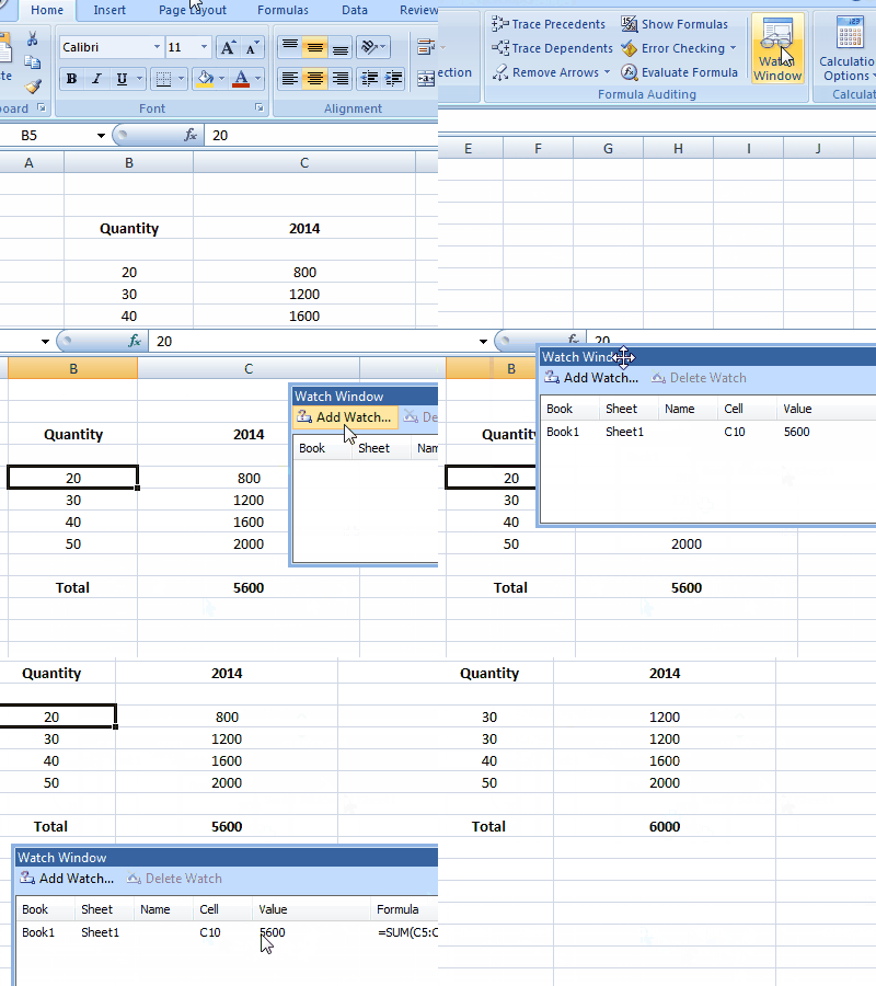
From now on, when you are changing the data, Watch Window shows the value changes of the dependent cell. Watch Windows keeps floating on the worksheet, and you can even resize it. You can even watch cells on the other worksheets also.
2] Round Off the Values to Thousands and Millions
It does not look good, and it looks weird, having the long numbers in the cell. So, it is better to format them and show them in a simplified way. I mean, show thousands in terms of “K” and millions in terms of “M.” To do so, select the cell or range of values, right-click on the selected region, and select “Format Cells.”
Now, click on the “custom” and type ###,”k” for rounding off to thousand and ###, “m” for millions. Click “Ok,” and you will see the simplified and rounded values. For example, value 22, 786.34 looks like 23k. This just changes the value looks, and the actual value remains the same. So, there will be no problem in using this.
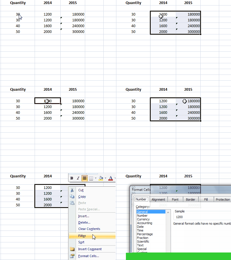
You can even format the axis shown in the chart in the same way. Select the axis you want to format and follow the process mentioned above.
Recommended: 5 Powerful and Most Useful Excel Features you need to know
3] Print Multiple Sheets on a single page
We will be in a situation where multiple worksheets should be printed on a single page. This can be done easily without the need for any add-on. For this, you need to have the camera on the Quick Access Toolbar (QAT). Click the down arrow of the QAT and select “More Commands”. From the dropdown “Choose commands from”, select “Commands not in the Ribbon”. Now, scroll down till you see “Camera”, select it and click on “Add >>” button, to add it to the QAT and click “Ok”. Now, the camera got added to the Quick Access Toolbar.
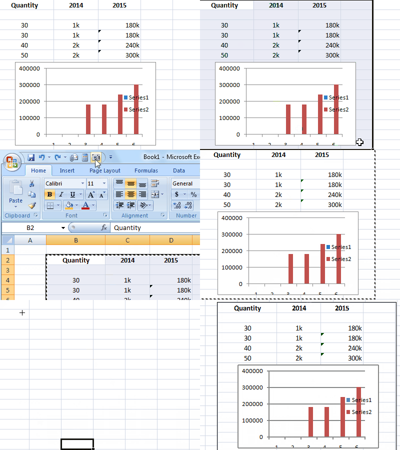
Now, select the first region or area which you want to print and click on the camera icon. Open a new worksheet and click where you want to paste it. You see that the selected region appears on the new worksheet.
Now, select the second region and do the same. Then follow this for all the regions you want to print on a single page. You need to remember one thing that, when you change the original value, then the value in the snapshot changes as it links to the original value.
4] Apply Table Format to your Excel Data
You can add the table style to your selected data. Select the data for which you want to add the table format and click “Format as Table” under the Home tab. Select the type of table you want, check the “My table has headers” and click “Ok” to see that table style is added to your Excel data. But, you also see that filters are added to the columns, and we want to get rid of it. To keep the range selected, click on “Convert to Range”.
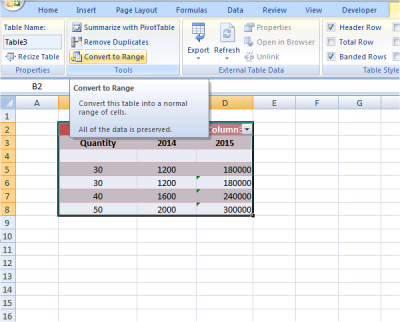
It asks “Do you want to convert the table to a normal range?” and click “Yes”. You will see that filters are removed, and the table format is applied to the data.
Read: Top 15 Financial functions in Microsoft Excel
5] Create a Custom List
It is always easy to select the value from the drop-down, rather than entering the value. You can create a custom data entry list in Excel to save time on entering. For this, first, have the values in one column that you want to be in the drop-down and select the location where you want to have the drop-down. Then, under the “Data” tab click on Data Validation > Data Validation. It opens up the Data Validation dialog box, select “List” from the “Allow” drop-down. In “Source” filed, specify the range which has values you typed initially and click “Ok”.
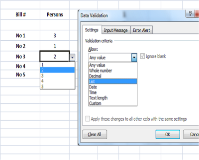
Now, click on the cell for which you added the Data Validation and it shows the drop-down arrow. Click on that arrow, and it shows all, in the list. Select the item to complete.
Read: How to insert Multiple Blank Rows in Excel at once.
These are some of the advanced Excel tips and tricks to do your complex tasks easily with just a few steps. Have you used any of the tricks mentioned in the list and do you have anything to add? Please, do share with us through comments.
thanks for this tips