In your school life, you have learned about average and the method to calculate it. The formula to calculate the average is very simple. You just have to add all the values in the given data and divide the result by the total number of values in the data. Moving average is also another type of average that has real-life applications. It has applications in many areas like the stock market, sales, etc.

Moving average is of three types, simple weighted and exponential. In this article, we will explain the methods to calculate all three types of moving averages in Excel.
Read: How to use MIN, Max, and AVERAGE Functions of Excel.
How to calculate Moving Average in Excel
We will calculate the moving average in Excel using two methods. In one method, we will use a built-in tool of MS Excel and in the other method, we will use formulae.
1] Using Data Analysis Tool Pack
In this method, we will use the Data Analysis Tool Pack in Excel to calculate the moving average. MS Excel comes with a tool to calculate simple moving averages. The Data Analysis Tool Pack is an add-in, which means you may not have it by default. We are listing here the steps to get this tool.
1] Click on the “File” option.

2] Select “Options.”

3] This will open a dialog box. Click on “Add-Ins.”
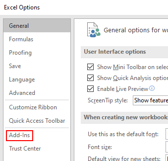
4] On the right panel of the dialog box, you will see a drop-down menu at the bottom. Select “Excel Add-ins” in the drop-down menu and click on the “Go” button.

5] Now select “Analysis ToolPack” and click on the “OK” button.
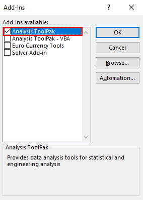
6] The above steps will install the Data Analysis Tool on MS Excel. You can view it in the “Data” tab.

Read: How to calculate the percentage difference between two numbers in Excel.
Now you are ready to calculate the simple moving average. To show you the calculation method, we have created sample data of varying temperatures for the first 10 days in a month.
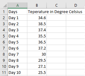
Please follow the below-listed steps to calculate the simple moving average using Data Analysis Tool Pack.
1] Click on the “Data” tab and select the “Data Analysis” option as shown in the above screenshot (see step 6).
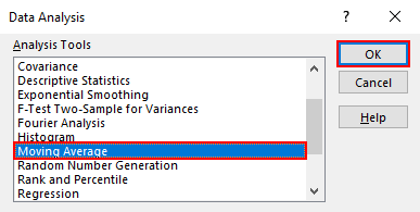
2] A small dialog box will open, where you have to select the “Moving Average” option and click OK. It is the simple moving average.
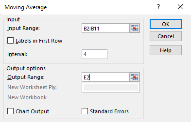
3] You have to enter the input range of the data for which you want to calculate the simple moving average. In our sample data, we have data ranges from cell B2 to cell B11. Therefore, we entered the range B2:B11. After that, enter the “Interval.” In the output range, you have to enter the address of the cell in which you want to get the output range. We selected E2. When you are done, click OK.
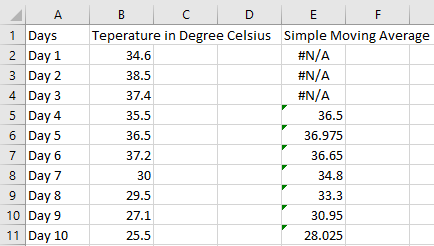
4] You will get the result. You can see in the below screenshot, the first three rows are showing #N/A error. This is because we have entered 4 in the “Interval,” which indicates that it is a 4 days SMA.
Read: How to Calculate Simple Interest in Excel.
In method 1 above, we have calculated the moving average with the help of a tool in Excel. But using method 1, we can calculate only the simple moving average. In method 2, we will calculate all three types of moving averages using formulae.
2] Calculation of Simple Moving Average (SMA) using Formula
We will take the same sample data here.
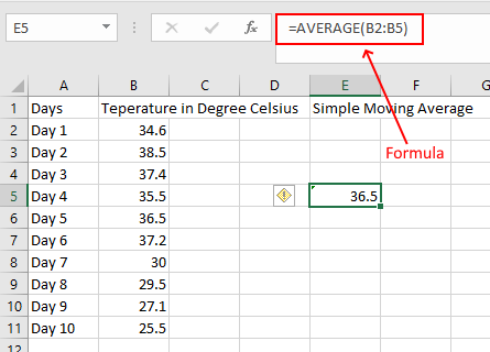
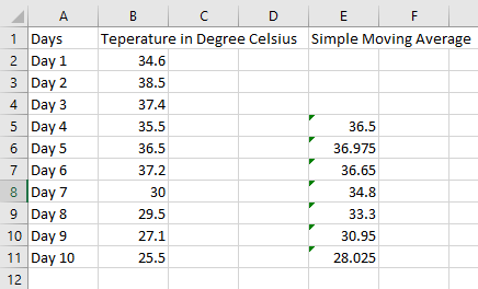
1] If you want to calculate the 4 days SMA, you have to enter the following formula in the cell that lies on row 5 (Day 4). After entering the formula, press “Enter.”
=AVERAGE(B2:B5)
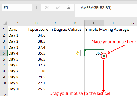
2] Now, hover your cursor on the bottom right corner of the selected cell. When your cursor changes to the “Plus” icon, press and hold the left click of your mouse and drag it to the E11 cell. This will copy the formula to the other cells.
3] You will get your result.
Read: How to calculate the area of a Rectangle, Triangle, or Circle in Excel.
3] Calculation of Weighted Moving Average (WMA) using Formula
Let’s calculate the weighted moving average. Again, we are taking the same sample data. To calculate the WMA, you should have the weights assigned to the particular values. The formula to calculate the weighted moving average is:
WMA = [(Latest value * weight) + (Previous value * weight) + ...] / (Sum of all weights)
We are calculating here 3 point WMA with 70% weight is assigned to the latest value, 20% to the value just before it, and 10% to the value before the second one. According to this data, you have to enter the following formula in the E4 cell.
=(0.7*B4+0.2*B3+0.1*B2)/(0.7+0.2+0.1)
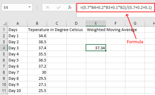
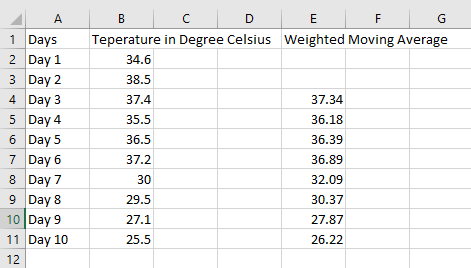
The first two cells are empty because we are calculating three-point WMA. Now, drag the cell to the last cell as we have done before in SMA calculation. You will get your result.
Read: How to calculate Median in Excel.
4] Calculation of Exponential Moving Average (EMA) using Formula
To calculate EMA, we should have the first EMA value, which we get by calculating the SMA and the weight multiplier or smoothing constant (K). The basic formula to calculate the EMA is as follows:
EMA = Latest Value or Today's Value * K + Yesterday EMA Value * (1 - K)
1] Let’s take the same table in which we have calculated the SMA. In this example, we have taken K = 0.3. The first EMA value is equal to the first SMA value. We are calculating here the 4 days SMA and EMA values.
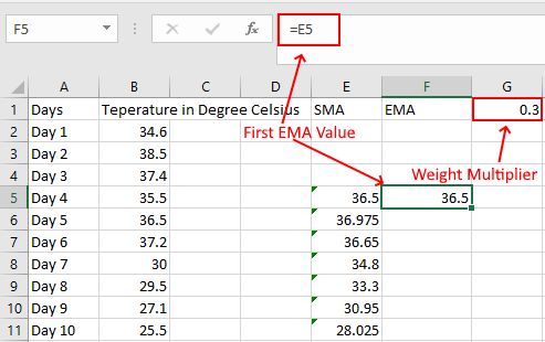
2] Now apply the following formula to the cell F6.
=B6*$G$1+F5*(1-$G$1)
Do note that, we have locked the cell G in the above formula because we need the same value of K for all EMA calculations.
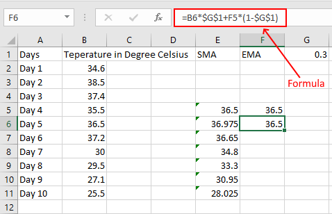
3] Now, Drag the cell to copy the formula to the remaining cells.
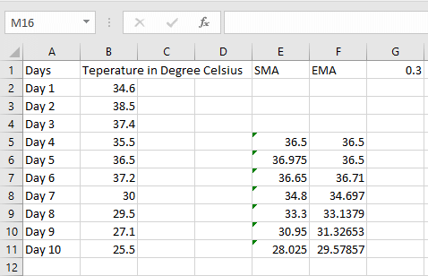
That’s it, we have calculated all three types of moving averages in MS Excel. We hope you enjoyed the article.
You may also like: How to calculate Grade Point Average or GPA in Excel.
Leave a Reply