Microsoft Excel can be used for budget calculations, Tax calculations and for many other purposes. You can use it as another form of calculator due to the features it provides us. You can even make use of Excel to calculate the difference between two times. It helps calculate the number of hours an employee worked between the given start and end time. A whole record of employee working hours can be maintained using Excel which helps us to calculate wages or salaries to be paid for an employee.

Do you think it is very easy to calculate the time difference as it is just subtracting the end time from the start time? If you just go ahead and do the same, you will face two problems. Let us see what are they, and how can we handle them.
Calculate Time Difference in Excel
It is tough to calculate the difference between two times in Excel. But with a little bit of trick applied, we can achieve the result we want. Just follow this article till the end and there on you can calculate time differences in Excel perfectly. Here we go!
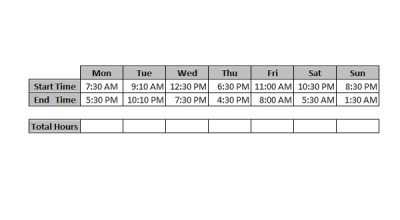
Just consider the sample data as below,

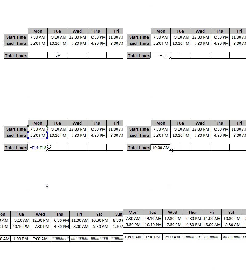
So, as discussed if we just try with subtracting the ‘End Time’ with the ‘Start Time’, you will be facing two problems and let’s see what are they.

You can see that result got appended with ‘AM’ or ‘PM’ which is not expected by us. The second problem is it shows hash errors. As we performed direct subtraction, the result might be negative in some cases and as the time should not be negative, Excel shows it as hash errors.
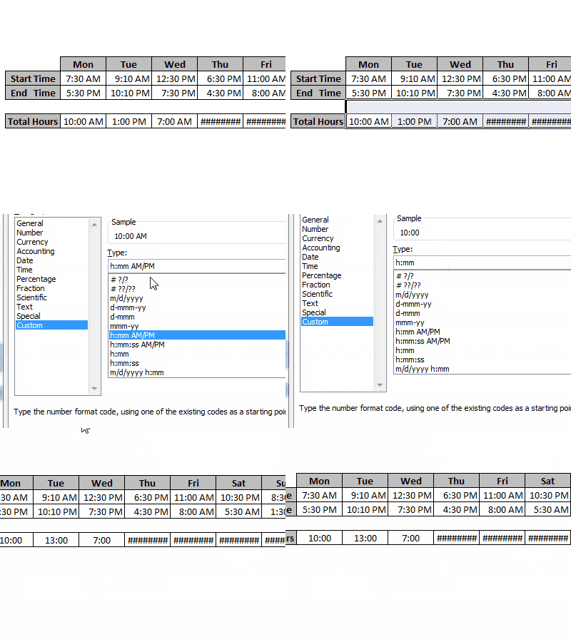
We can solve the first problem by changing the number format by following the simple below steps
- Select the cells which have the result (Total Hours in our case) and press ‘CTRL+1’ to open the format cells dialog box.
- Click on the “Custom” option and in the “type” field enter “h:mm” and click “Ok”.

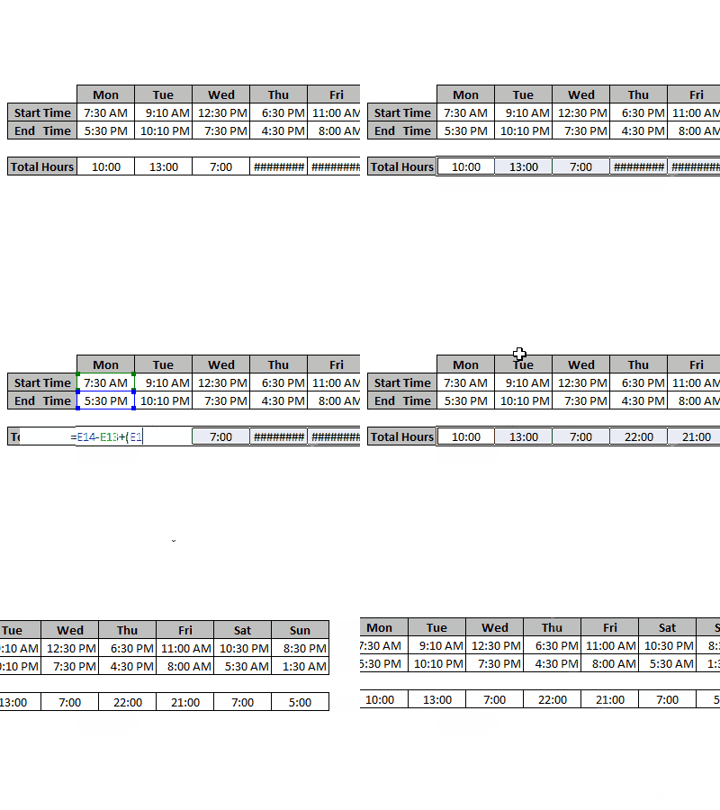
In this way, you can get rid of the first problem. This is somewhat satisfying but even though it is not the complete solution which we are looking for. We still need to remove the hash errors in Total Hours calculated. To solve the second problem, you need to change the formula which you used in the first step (End Time – Start Time i.e. ‘E14-E13’). Select the Total Hours row and press ‘F2’ to change the formula. Make the formula as follows-
E14-E13+ (E13>E14)
Now, instead of pressing the Enter, just press ‘CTRL+Enter’ so that the result is applied to all the selected cells in a single shot. This way we can avoid changing the formula for every cell.

We all know that 24 hours system is being used by Excel. The main tricky part used here to solve the hash errors is adding the logical operation. By doing so we have overcome the negative result as “TRUE” is treated as “1” and “FALSE” is treated as “0”. Finally, the time difference does not show the negative values and else no hash errors anymore.
This is the simple, easy and perfect way to calculate time differences in Microsoft Excel.
Read: How to lock the Chart position in Excel
How do I calculate the time difference in Excel in 24 hours?
Once you have calculated the time difference, you can right-click on it, and then select Format. Then set the display time in 24 hrs format. However, if you calculate the time difference in number format, it will work differently i.e, 12:00 PM will be calculated to 0.05 because it’s half of a day.
Would not using the 24 hour clock be a simpler solution?
I mean using square brackets in the answer cell will give the same result, wont it?
Last sunday I worked Straight from 12:00 AM to 12:00 AM. The results is zero. How can I make to show 24 hours worked?
That is also a simple solution!
To handle such scenarios, we need to enhance the formula a bit I hope.