Most of us use To-Do apps to list down the tasks which we want to do on a particular day. This keeps us completing our tasks without any procrastination. But, if you are an Excel lover like me then we can use Microsoft Excel to create a checklist or To-Do list easily. We generally use checkboxes in Excel only while creating forms. But, in this article, I will let you know how to use checkboxes to create a checklist in Excel. Follow through to the end of the article to know how to do it.
Create a Checklist in Excel
I will take you through few series of steps so that it would be easy to understand. So, let us start without any ado.
1] Activate Developer Tab in Excel
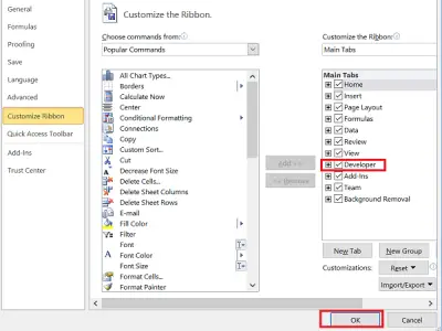
As a first step, you need to enable the ‘Developer’ tab in Excel. To do so, go to File and select Options. In ‘Excel Options’ dialog box, select ‘Customize Ribbon’ and on the right side check the box beside ‘Developer’ and click Ok. Now you could see ‘Developer’ tab on the Excel ribbon.
2] Prepare Tasks in Excel
Now, prepare a column ‘To Do’ and enter the tasks that you want to do. Say, I have added tasks from E7 to E9.
3] Add Checkboxes in Excel
It is time to add Checkboxes. Besides the ‘To Do’ column we need to add Checkboxes. So, for every entry in column E7 to E9, we need to add checkboxes from F7 to F9. To do so, first, click on ‘Developer’, click on ‘Insert’ and click the checkbox icon under ‘Form Controls’. Now, click on the Excel cell where we want to insert this checkbox and in this case it is F7.
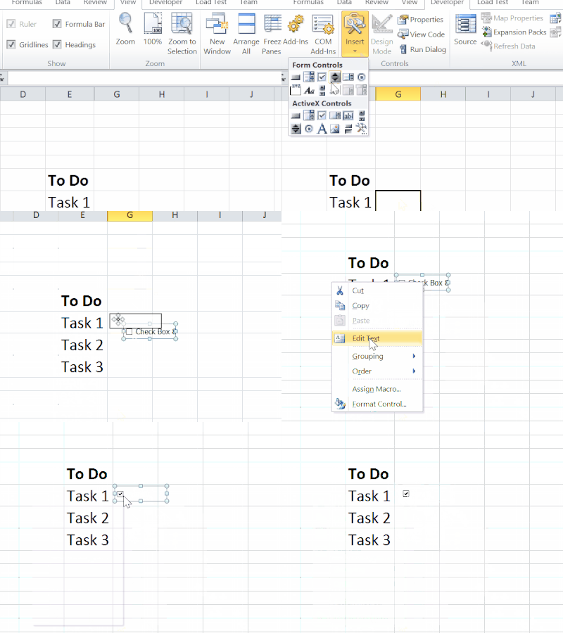
We can see that some default text was added along with the checkbox. To remove that, right-click on the checkbox, select ‘Edit Text’ and delete the text. Repeat this step for the remaining columns also (F8 and F9 in this case).
4] Assign a cell to each Checkbox
Now, we need to assign a cell to each checkbox so that when we tick and untick the checkbox, the values TRUE and FALSE are shown, respectively. To do so, right-click on the checkbox and click ‘Formal Control’.
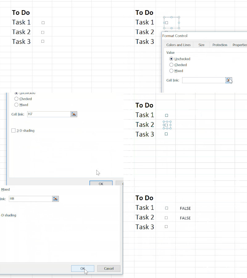
In ‘Formal Control’ dialog box under ‘Control’ tab give the address of the cell in ‘Cell link’ box which you want to assign to the checkbox. Let me choose the cell ‘H7’. Make sure that you give the cell address as ‘H7’ only and not in any other format. Repeat this step for the remaining checkboxes as well.
5] Apply Conditional Formatting
Select the tasks that you have added in previous steps, click on ‘Conditional Formatting’ under the ‘Home’ tab, and select ‘New Rule’. Now, select the rule type as ‘Use a formula to determine which cells to format’. In the condition textbox, we need to check the value of the cell, which gets updated when the checkbox is ticked as TRUE or not.
Next, click on ‘Format’ button, select ‘Strikethrough’ under ‘Effects’ and select a red color from ‘Color’ dropdown and click ‘Ok’. Repeat this step for every task you entered.
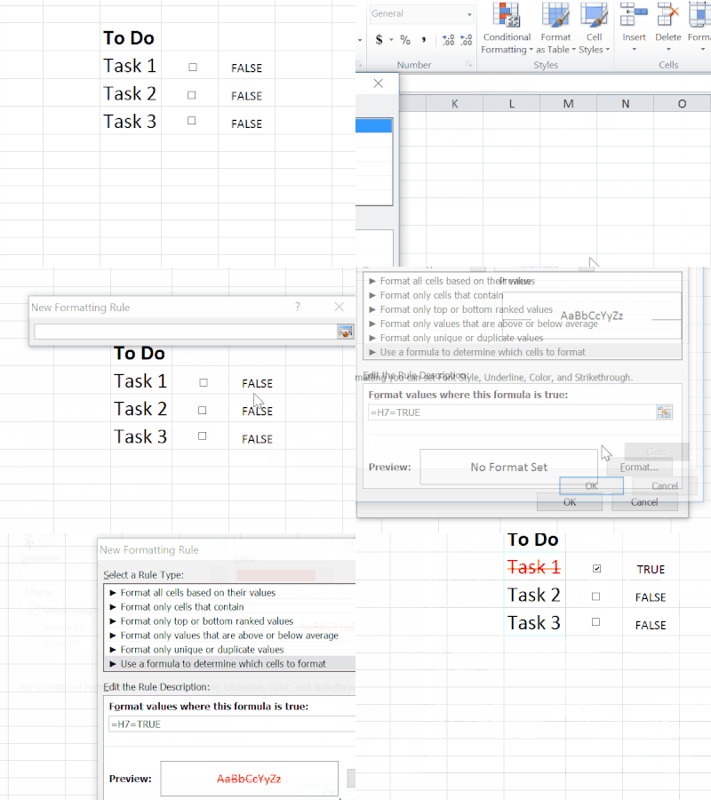
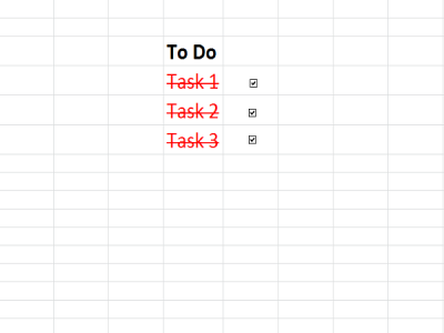
Now, it is time to hide the column that gets updated for every tick and untick a checkbox so that the Excel sheet only has tasks and checkboxes. So, now, when you tick the checkbox beside the task, you can see that the text gets red color, and it strikes the text that mentions that the task has been done.
This is the simple way to create a checklist in Excel.
See this post if you would like to know how to make a Checklist in Word.
