How to delete Pivot Tables in Excel

One of the best features in Microsoft Excel is the Pivot Table, believe it or not. There is no need to learn any formatting or coding to create hundreds of rows of data along with quick summaries of everything. You just need to know how to drag and drop and how to create a Pivot Table.

Now, a lot of people know how to create a Pivot Table, but unfortunately, many have no idea how to delete one. In most cases, after a Pivot Table is created and populated with content, there are few reasons for it to be deleted, so we can understand why some folks are not well versed in deleting tables.

How to delete Pivot Tables in Microsoft Excel

Deleting a Pivot Table is not difficult. In just a few steps, the task will be completed and right away you’ll become an expert. Now, we will discuss how to delete the Pivot Table and keep the data or delete the tables along with the data. The choice is yours as to what you want to accomplish. There are 3 scenarios:

1. Delete Excel Pivot Tables and keep the data
2. Delete the Pivot Table along with the data
3. Delete the data and keep the Pivot Table

1] Delete Excel Pivot Tables and keep the data

In some situations, the user wants to delete the Pivot Table but at the same time, retain the data. This might seem complicated, but believe us, it is not.

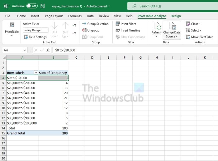
• Select a cell from within the Pivot Table
• Look to the Ribbon and click on the Pivot Table Analyze tab.
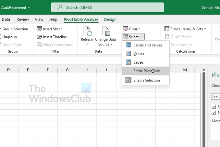
• Click on the Select button located within the Actions category.
• From the dropdown menu, please click on Entire PivotTable.
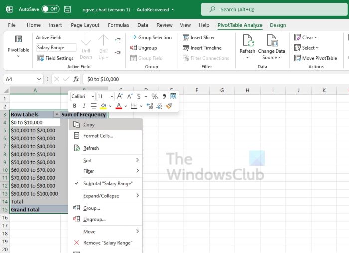
• Right-click on the selected Pivot Table.

• Select the Copy option right away.
• The next step, then, is to click on the Home tab.
• From there, click on the Paste option.
• Via the Past Values section, choose the first option.

The Pivot Table should now be gone, but the data remains the same, and that’s a good thing.

2] Delete the Pivot Table along with the data

For those who want to delete the Pivot Table along with the data, then you can be sure it is something you can do. Let us discuss how to get this done the easy way.

• Click on one of the Pivot Table cells.
• From there, select Pivot Table Analyze
• From the Actions category, click on Select.
• A drop down menu will appear.
• Via that menu, select Entire PivotTable.
• Click the Pivot Table to select it.
• Finally, hit the Delete key to have it removed forever.

If you want, you can move to create a new Pivot Table at any time with new data to populate.

3] Delete the data and keep the Pivot Table

In certain situations, the user might want to keep the Pivot Table but get rid of all the data. The question is, how to do this without having to manually remove each piece of information?

• Click on a cell located in the Pivot Table.
• After that, you must click on the Pivot Table Analyze tab.
• Look to the Actions category and select Clear.
• Finally, click on Clear All.

All data from within the Pivot Table should now disappear, leaving an empty table for new data whenever you’re ready.

Read: How to create Formula to Add, Subtract, Multiply or Divide in Excel

What is a Pivot Table in Excel used for?

If you want to summarize large and organize large amounts of data,  your best bet is to use Pivot Tables. They are great for analyzing numerical data in detail and answering unanticipated questions about the relevant data. It allows you to quickly group and analyze data by different dimensions, such as category or date. You can also create charts and graphs that visually represent the data.

Where are Pivot Tables in Excel?

If you want to find the Pivot Tables in Microsoft Excel, click the Insert tab. From the Tables group, please select Pivot Table and move on from there. You can also quickly press the keyboard shortcut Alt + N + V to access the “Create PivotTable” dialog box. From what we have gathered thus far, the four Pivot Table fields are Filters, Columns, Rows, and Values.