Excel spreadsheet is the premiere application used by many industries to frame business plans, create financial reports, produce budget reports, etc. In simple words, Excel spreadsheets are used to systematize your work life. While Excel is a powerful spreadsheet tool, one can ever get to work, mastering Excel can be time-consuming and it would probably require some patience to work with Excel spreadsheets.
Excel Tips to Save Time and Work Faster
Managing and Calculating data in Excel with advanced formulas requires your through skills in financial analysis and is way more critical than we imagine. Some jobs have monotonous steps which will require you to repeat unnecessary tasks over and over again which will waste your time.
Microsoft Excel does tedious jobs easily. Whether it’s repeated tasks or managing data cleanly, Excel does it well. However, most people do not know many Excel features. Knowing those hidden tips and features helps us complete our work faster and save a lot of time. Today, I will share some Excel tips to save time and complete your work faster on your Windows computer.
Microsoft Excel time-saving tricks
It is important to take your Excel skills to the next level to make sure that your methods of using spreadsheets are churning out maximum efficiency. Excel has many integrated features that allow you to get your work done quicker. You can master some of the tips and tricks for most frequently used steps in Excel to improve your efficiency while working with Excel and save your precious time. In this article, we outline some of the tips which you can include in the daily workflow that can liberate you from doing repetitive tasks and help save your time while using Excel.
We may be facing small problems like creating multiple lines in a single cell or printing multiple worksheets on a single paper. We follow different techniques to do this, which might not be as efficient as we might want them to be. This article will let you know how to do such tasks easily to save your time so that you can complete your work in a faster way.
1. Use AutoFill
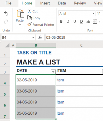
Auto Fill is a very useful feature that will automatically fill a series of cells based on the pattern of previous cells. Suppose you want to enter a column with names of a month, simply enter Jan. Select the cell and drag it down. The Autofill magically fills in the month names based on the previous pattern.
2. Use Flash Fill
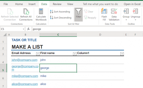
Flash Fill automatically combines and extracts data based on the data pattern entered in the first column. For example, if your first column has abc/123/xyz and you want to extract the value 123 into the second column. Simply enter the data in the first cell. By the second cell, excel will know the pattern and displays what you want them to look like by simply using Flash Fill in the Data Tools group.
In the same way, you can flash fill to combine the data. .For example, if you have email addresses in the first column, you can use Flash fill to create the first column by entering the correct email pattern and first name in the second column. In simple words, if you want to extract or combine the data, simply click on Flash Fill in the Data Tools session by typing the pattern how you want them to display.
3. Use the F4 key to automate the repetitive task
The F4 key is the most popular keyboard shortcut used which will save your time while doing repetitive work. If you are repeating the same steps over and over again, you can automate the repetitive tasks by using the F4 key. The F4 simply repeats your last action or command. Additionally, you can use F4 key To close the workbook and Excel window. Press Ctrl+F4 to close the workbook and use Alt+F4 to close the Excel.
4. Use Ctrl keyboard shortcut
There are many keyboard shortcuts which provide the most efficient and faster ways to complete a repetitive task.
- Ctrl+Shift+down arrow – selects all the data in the column below the cell.
- Ctrl+Shift+up arrow– selects all the data in the column above the cell.
- Ctrl+Shift+right arrow– selects all the data to the right in the row
- Ctrl+Shift+left arrow– selects all the data to the left in the row
- Ctrl+Shift+ End – jumps the cursor to the lowest right cell containing a data in a worksheet and selects ever cell with data in between the first cell you want to select and the lowest right cell with data.
To know more about the CTRL keyboard shortcuts, check the list on office.com.
Read: Top 15 Financial functions in Microsoft Excel
5. Add a note to explain formulas and functions using N()function
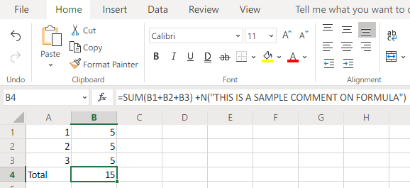
You can annotate cell with explanatory notes which will help you to remember and explain complex functions and formulas to other spreadsheet users. To include comments to the complex formulas simply add +N(“your comments “) at the end of the formula. For example, a cell with formula =Sum(B1:B2: B3) +N(“your note on formula”) displays both comments and formula when you click on that cell.
6. Use Paste specials for quick calculations
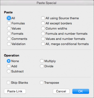
You can perform quick calculation like addition, subtraction, multiplication or division in the spreadsheet by using Paste Special instead of using formulas. This feature is easy to use and is extremely useful for small calculations to get your work done quicker. For example, if you have a column with a list of numbers which you want to divide it by 100. Type 100 in a cell and copy it. Select the list of the number which you want to divide by 100 and click Paste special. In this dialogue box, select the Divide option. This method will instantly divide all the selected numbers by 100.
7. Multiple Lines in a Cell
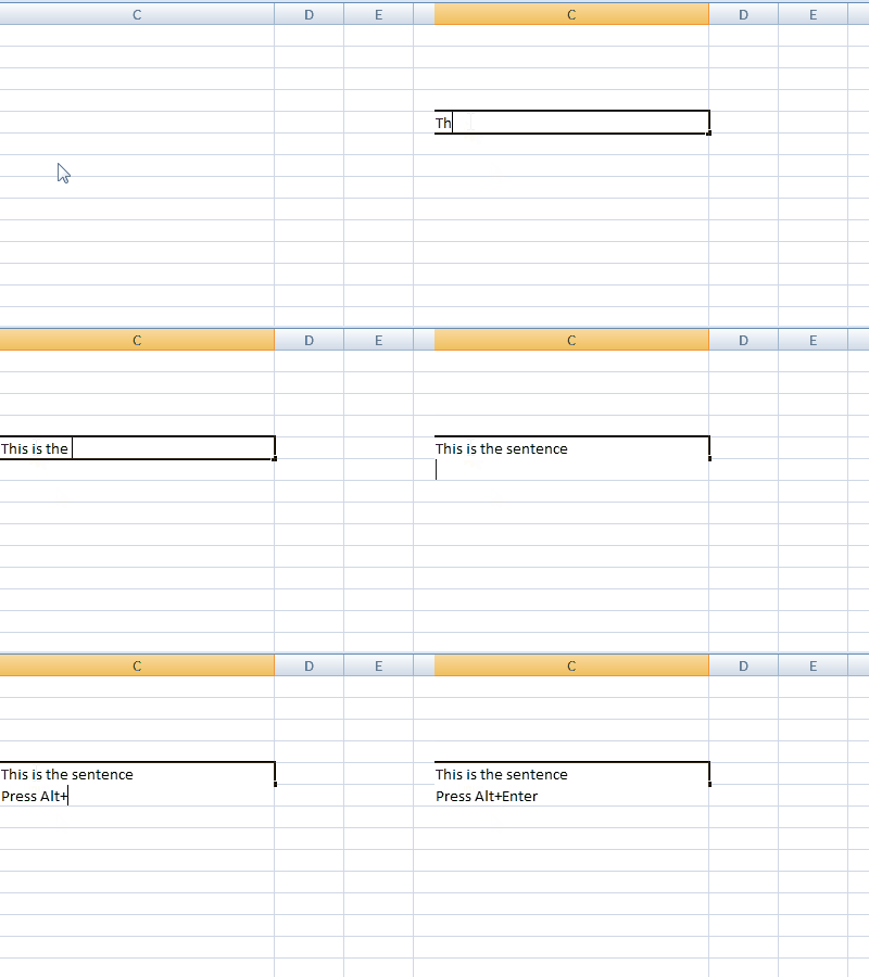
While filling the Excel sheet, sometimes we need to have a lot of information in a single cell. For example, if you want to write the address in a cell, then it needs to be on multiple lines within a cell. Then, if you press the “Enter” button, the control moves to the next cell, but that is not what we want. Press Alt + Enter to move the cursor to the next line of the same cell. This would be the savior for having multiple lines in a single cell.
8. Add Cell Values Quickly
If you want to add values or the average value of multiple cell values, then there is no need to use the formula. To get these basic things done, select the cell, press “Ctrl” key, and select the cells which you want. On the status bar which is at the bottom of the Excel sheet, you can find the Sum, Average, and other values being calculated. If you want to see other values, just right-click on the status bar and select the value you want to see.
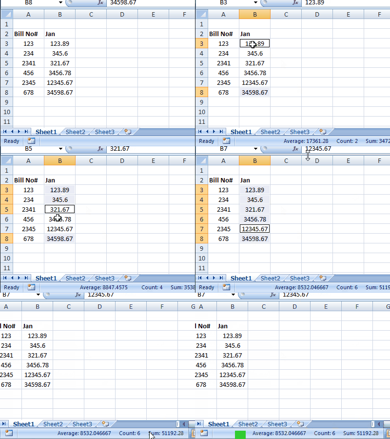
You can add values like Minimum, Maximum, Numerical Count (selected cells containing the numerical values) and many more like this.
9. Create Chart Templates to reuse
Creating the same sort of chart, again and again, is repetitive work. For example, if you want to create a chart for sales data of the entire month, it is better to create the chart template and use the same template every time you want to use the chart. To create and reuse the chart template, follow these steps.
- Select the required data and insert the chart in a regular way.
- Format it as you want. Add or remove gridlines, data labels, trend lines, and everything you want.
- After formatting the chart as you want, select the chart and click on “Save as Template” under the Design tab.
- Now, save the chart with “.ctrx” extension. The default location to save the chart template is C:\Users\Username\AppData\Roaming\Microsoft\Templates\Charts and save the chart template in this location itself. If needed, you can even choose your destination.
- Now, to reuse the chart template, select the latest data and head over to the “insert”, in “Charts” section, go for “Other Charts” and “All Chart Types”. Click Templates and select the template you want. This creates a chart for the latest selected data.
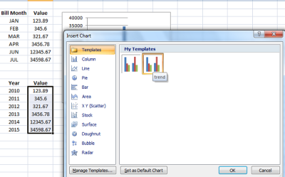
By using the chart template, it saves a lot of time, and there is no need for creating the chart as you want from the beginning.
10. Create a Chart from different cell values
We can create a chart from cell values that are not adjacent. As we already know that, we can select values present in various cells by holding the Ctrl key, then in the same way select values which are not the adjacent cells and then insert the chart. For example, if you have headings in the first column and values in the fourth column, hold the Ctrl key and select the first column and fourth column, then insert the chart.
11. Use Names in Formulas to Understand Easily
Having a name is always easy to recognize. In the same way, having a name to a particular cell or range of data and using it in formulas is easy to understand the formula well. For example, Commission * B5 is easy to understand than C2*B5. To do so, select the cell or range of data and under “Formulas” tab click on Define Name. It asks you to enter the name and check the reference cells before entering the name and click “Ok”.
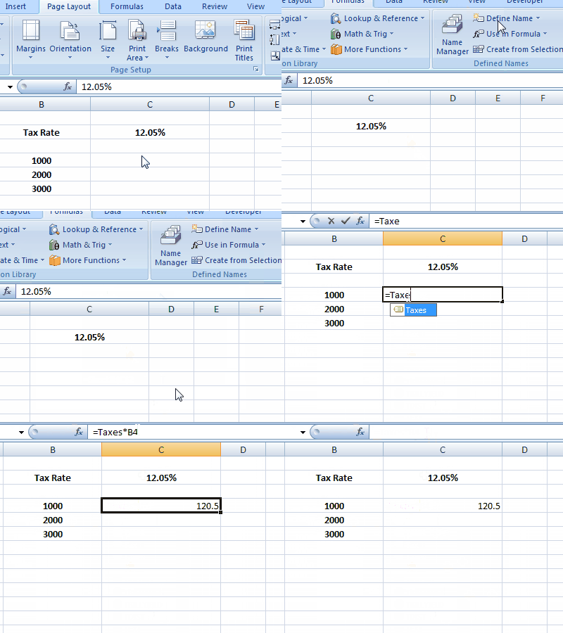
Say I created the name “Commission” by selecting a particular cell, then when I use Commission*B5, it refers to the cell value which was named Commission.
Read: Make the best use of Name Box in Excel.
Note: Name should start with a character and can also start with an underscore. It should not start with a number, and it should not have spaces.
All the created names can be seen from the Name Box. Click on the drop-down arrow in the Name Box, and it shows the list of names created. Select the name, and it takes you to that particular region or area in the worksheet.
Read: Excel Online tips.
These are some of the Microsoft Excel tips for saving time and helping you to complete your tasks easily and quickly. If you have anything to add, please do share with us through comments.
Which tricks do you use most frequently to save time while working in Excel? Do share in the comments below.
Now read:
- 10 most useful Excel Tips and Tricks for beginners
- Advanced Microsoft Excel Tips and Tricks for Windows users
Leave a Reply