Microsoft Excel makes it simple to retrieve stock market prices. Its Stock data type is connected to an online data source that allows you to access rich, interesting information you can work with and refresh. Let’s see how to get Stock Quote in Excel.
Get real-time Stock Prices in Excel
You can retrieve stock quotes in Excel by using the MSN MoneyCentral web query – but things have changed a lot now. The new system provides rich, interesting information that you can work with and refresh instantly! The way to do it is like this:
- Create a table
- Enter a ticker symbol
- Let Excel find the match for your entries
- Add a column to extract more information
- Space the entries in the table
Since data like the share price constantly changes, refreshing the connection always gives you the latest information.
1] Create a table
For this, go to ‘Insert’ tab and select ‘Table’.
To add a stock price to your Excel worksheet, convert text into the ‘Stocks’ data type. Following that, you can choose another column to extract relevant details, like the stock price, change in price, and so on.
Enter the text that describes the company name or fund name into each cell. Alternatively, you can enter a ticker symbol.
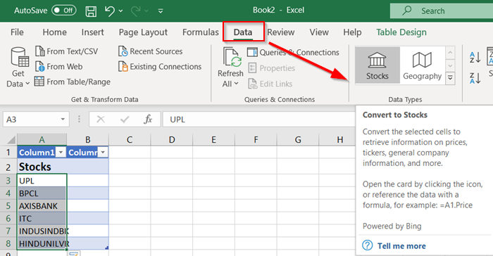
Select the cells and go to the ‘Data’ tab. Then click ‘Stocks’.
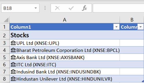
If Excel finds a match between the entries you’ve made in the cells, and its online sources, it will readily convert the text to the Stocks data type. This can be verified by when ‘Linked record icon for stock’ becomes visible to you.
2] Add column to extract more information
Now, choose one or more cells with the data type. The ‘Add Column’ button should appear.
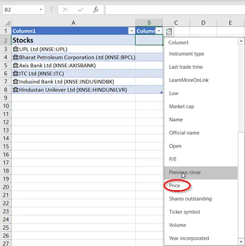
When seen, click that button and then click a field name to extract more information. For stocks, you might be interested in the most important determinant: Price.
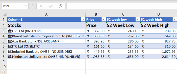
Click the ‘Add Column’ button again to add more fields. For instance, you can track the performance of a stock over a period of weeks, months, or years.
To space the entries in the table, select all columns and go to ‘Home’ tab.
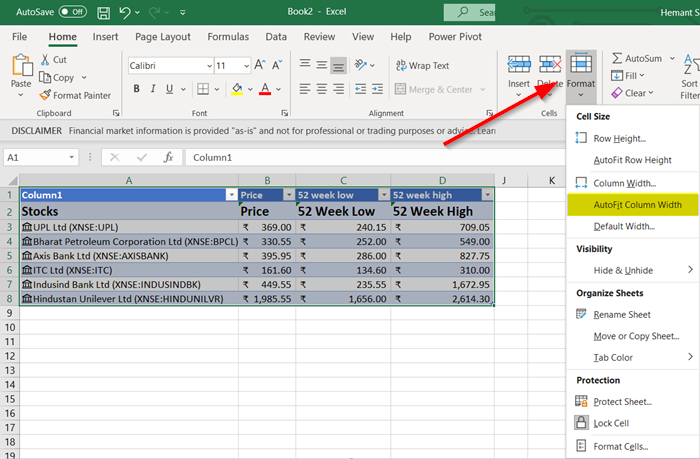
Then, go to the ‘Cells’ section and hit the ‘Format’ down-arrow button.
Select ‘Auto-fit column width’ and you are done!
So cool!