HLOOKUP is a Function in Microsoft Excel that looks for values in a Horizontal list. The HLOOKUP function searches for values Horizontally in the top row of a Table or Array, and returns a value from the column of the same Table or Array of value, and returns the value from a row you specify. The H in LOOKUP stands for horizontal. The difference between the VLOOKUP and HLOOKUP is that the VLOOKUP searches for columns and the HLOOKUP look for rows.

Function Syntax for HLOOKUP
- Lookup_ Value: The value to be found in the first row of the table.
- Table array: The table where the information is looked up. Use a reference to a Range or Range Name. The value in the first row of Table_ Array can be text, numbers, or logical values. If the Range_ Lookup is TRUE, the values of the first row of the Table _Array must be arranged in ascending order, for instance, A-Z. HLOOKUP will not give the correct value if the Range_ Lookup is FALSE; Table _Array does not need sorting.
- Row _index_num: Row_ Index_Num must be required. The row number in Table_ Array from which the matching value must return. If the Row_Index_Num is less than one, the HLOOKUP function will return the #Value! Which is an error value. If the Row_Index_ Num is greater than the number of rows on Table_ Array, HLOOKUP will return the #REF! Error Value.
- Range _Lookup: Range_ Lookup is optional. It is a logical value that specifies whether you want HLOOKUP to find an exact match or an approximate match.
The HLOOKUP function should be used when the comparison values are in a row across the top of a table of data, and you want to look at a specified row. In this tutorial, we will explain how to create an HLOOKUP function.
How to use the HLOOKUP function in Excel

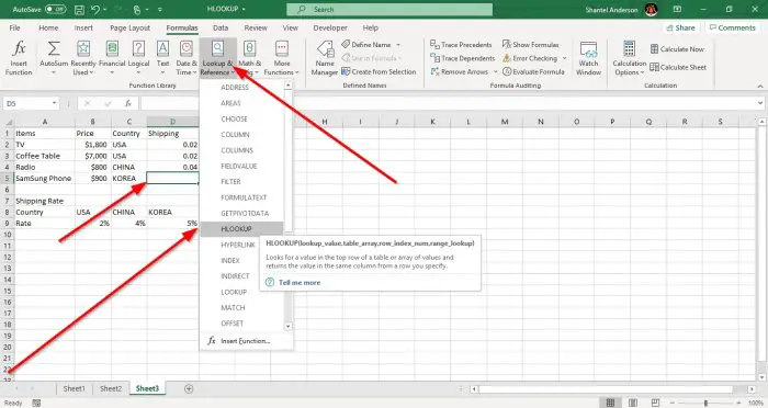
In this tutorial, we want to Lookup the Shipping Rate of each item in the table.
Click the cell where you want to place the function’s result, then go to the Formulas tab and select the Lookup and Reference Tool in the Function and library Group, in the drop-down menu.
Choose HLOOKUP, and a Function Arguments dialog box will appear.

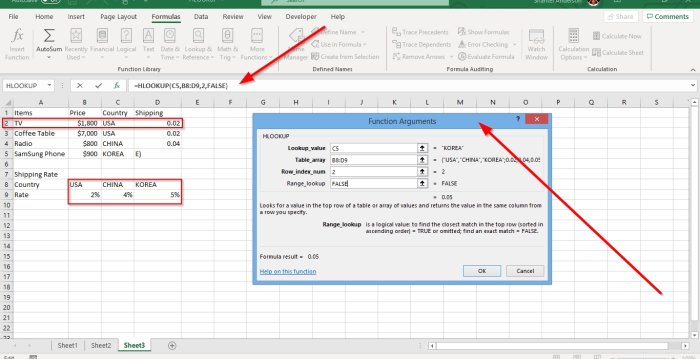
In the Function Arguments dialog box, type the cell you want to change in the Lookup_ Value text box.
In the Table_ Array text box, we type B8:D9; because this is the Range of cells we are looking at.
When it comes to the Row_ Index_ Num, select a row. For instance, in the image above, you will see that the table’s data starts from row 2.
In the Range Lookup, type False because you want an exact match. Select Ok. You will see your result.
The Other Option is to type the formula =HLOOKUP (lookup value, table _array, row_ index_num, [range lookup] and input your data.
I hope this helps.