If you want to know how to add a tooltip in Excel and Google Sheets, then keep reading this article. Both Microsoft Excel and Google Sheets allow adding a tooltip to a cell value to show readers a message regarding the data or information given in the cell.
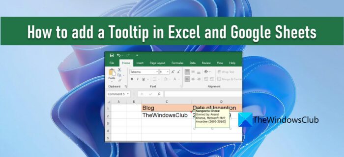
Tooltips are small windows that pop up when you select or hover over a cell. Interestingly, there is more than one way to display tooltips in spreadsheets. In this post, we will show you how to add a tooltip to a cell value in both Microsoft Excel and Google Sheets.
How to add a Tooltip in Excel and Google Sheets
To display a tooltip, you may use Comments, Notes, Data Validation Help Text, or Screen Tips. Let us see how they work in Excel and Google Sheets.
1] Adding a Tooltip in Microsoft Excel
A] Adding a Tooltip via Comments
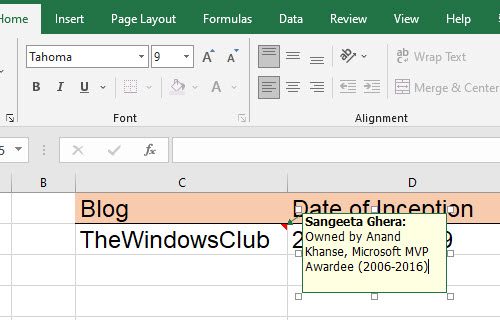
To add a tooltip in Excel through comments, follow the steps listed below:
- Right-click on the desired cell and select Insert Comment. Alternatively, you can select the cell and press the Shift+F2 key combination.
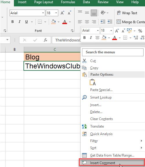
- A textbox will appear. Write the text you’d like to show as a tooltip.
- Click anywhere outside the cell.
A red-colored triangle on the top-right corner of the cell indicates that the comment has successfully been added.
Note: In Excel for Microsoft 365, the ‘comments’ feature will allow you to initiate a discussion using a thread, while you may still add a simple annotation to the cell through the ‘notes’ feature. More on this in the Google Sheets section.
B] Adding a Tooltip via Data Validation Input Message
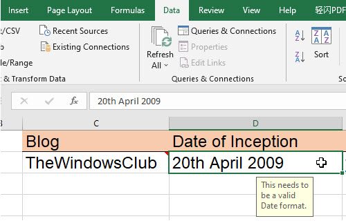
To add a tooltip in Excel through the Data Validation Input message, follow the steps listed below:
- Select the desired cell.
- Go to the Data tab.
- In the Data Tools section, click on the Data Validation dropdown.
- Select the Data Validation… option.
- In the Data Validation window, switch to the Input Message tab.
- Enter the text you want to display as a tooltip in the Input message textbox.
- Click on the OK button.
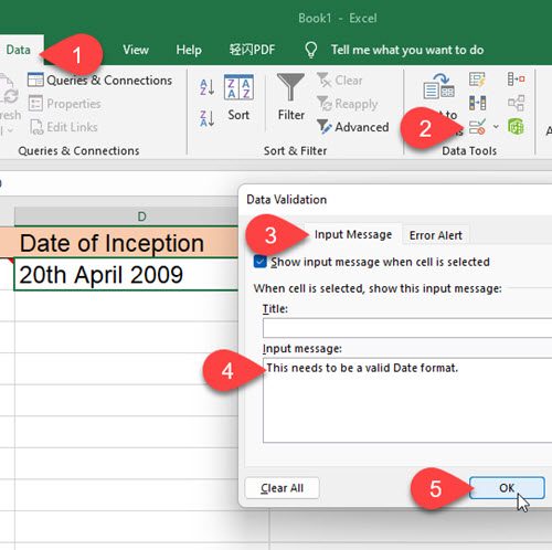
The tooltip will appear when the cell is in focus.
C] Adding a tooltip to hyperlinks via ScreenTip
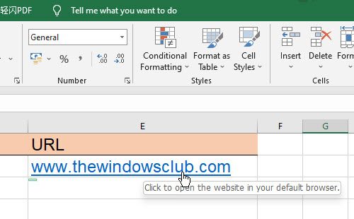
When you mouse hover on a hyperlink in MS Excel, it automatically shows a tooltip. If you want to add a custom tooltip to such links, follow the steps described below:
- Right-click on the cell and select the Edit Hyperlink… option.
- In the Edit Hyperlink window, click on ScreenTip… button.
- Enter the tooltip in the ScreenTip text textbox.
- Click on the OK button.
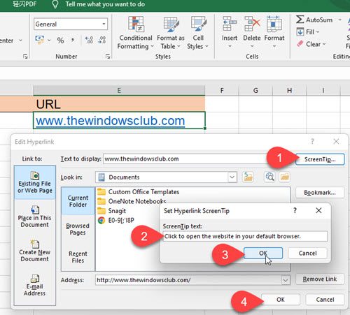
Your custom tooltip will now appear when you mouse hover on the cell, instead of the default tooltip text.
2] Adding a Tooltip in Google Sheets
A] Adding a Tooltip via Notes
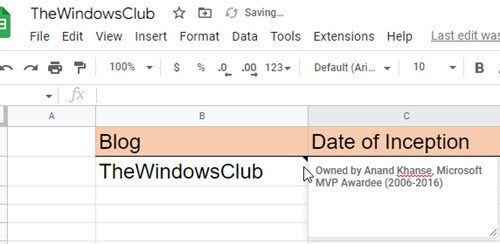
Notes allow you to attach an annotation with a cell value in Google Sheets. This works similar to the Comments feature in Excel. To add a tooltip to a cell value in Google Sheets via notes, follow these steps:
- Select the desired cell.
- Right-click on it and select the Insert Note option from the context menu.
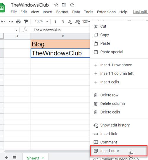
- Enter the tooltip in the textbox that appears.
- Click anywhere outside the cell.
Next time you hover over that cell, you will see the tooltip.
Also Read: How to Highlight Duplicates in Google Sheets.
B] Adding a Tooltip via Comments
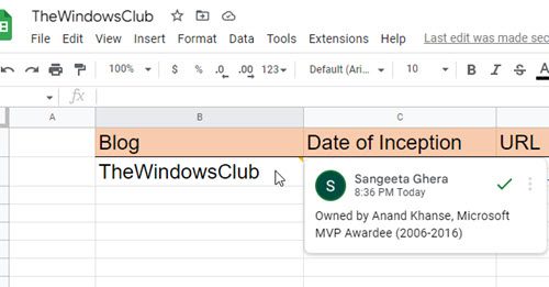
Comments in Google Sheets is a more comprehensive feature that allows multiple users (that share the same spreadsheet) to add their respective comments on the same cell value. This creates a thread of comments that can be used for discussions. The name and profile picture of the user appears with each comment. If you want, you can use comments to add tooltips to cells in Google Sheets. Here’s how to do it:
- Right-click on the desired cell and select Comment.
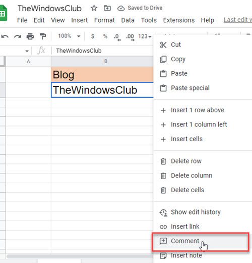
- Write the tooltip text.
- Click on the Comment button.
Now when you mouse hover on that cell, you will see the tooltip. And when you select the cell, you will be able to add more comments to the thread.
C] Adding a Tooltip via Data Validation
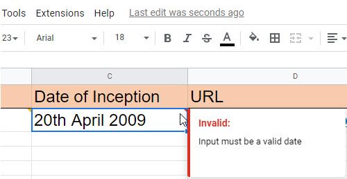
Google Sheets lets you display a tooltip upon entering invalid data in a particular cell. To show these tooltips, you have to apply a data validation rule to the cells.
- Select the desired cell (or a range of cells).
- Select Data validation from the Data menu.
- Set data validation Criteria. For example, you can set Date > Is valid date.
- Select Show warning in the On invalid data field (The Show warning option allows invalid input in the cell but shows a warning message, whereas the Reject input option rejects the invalid input).
- Click on the Save button.
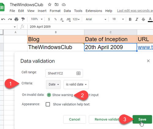
Now when the user enters incorrect data in the cell, a red triangle will appear on the top-right corner of the cell. When he hovers over that cell, the tooltip message will be displayed.
Please note that the ‘Show validation help text’ feature works in the case of the Reject input option only.
This pretty much sums up different ways to add a Tooltip in Microsoft Excel and Google Sheets. Hope you find this helpful. Do share in the comments if you have any queries.
How do I add a tooltip to an Excel spreadsheet?
There are multiple ways to add a tooltip in Microsoft Excel. The easiest is to select the cell, right-click on it, and choose the Insert Comment option. You may then enter the tooltip text in the textbox that appears. The tooltip will also display the name associated with your Microsoft office profile. Apart from this, you can display a tooltip based on data validation, or display a screen tip over a hyperlink as described in this post.
How do you hover text in Google Sheets?
You can hove text in Google Sheets using tooltips. You can add a tooltip in Google Sheets using the built-in Comments and Notes features. The Notes feature allows you to display a simple annotation (or tooltip text) over a cell value, while the Comments feature lets you start a conversation with other users who share the same spreadsheet. The difference is, when you use Comments to insert a tooltip, your name and profile picture will be displayed along with the tooltip, while with Notes, nothing except the tooltip text will be displayed.
Read Next: How to Export or Import Data from Excel to Google Sheets.