Making selective cells stand out in a Microsoft Excel spreadsheet is possible by adding a border. For example, you might consider calling attention to the result of a particular calculation. Borders can be created in several different ways. Users can create borders that are comprised of solid lines or multiple dashes. Let us see how to add a Border in Excel.

How to add Border in Excel
To add a Border to one or more Cells in Microsoft Excel by clicking follow these steps:
- Open an Excel spreadsheet
- Select the cell or cells
- Click on the Borders button
- Select an option from the Border menu
- Change the color.
To begin, open the Excel spreadsheet.
The next step is to select a single cell or a group of cells to which the border must be applied.
In order to select a cell, all you have to do is click on the cell.
When it comes down to a group of cells, click one of the cells. From there, hold the Shift key, then use the arrow keys to enlarge the selection.
Alternatively, you could press and hold the left mouse button, then drag the cursor to increase the range of all selected cells in the spreadsheet.

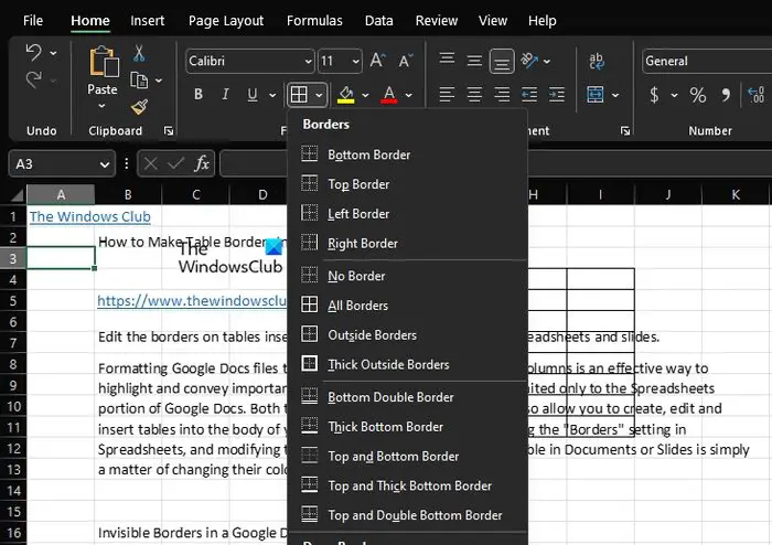
Next, click on the Home tab located in the upper left section and look to the Font group via the Ribbon, and then click on Borders.
A drop-down menu for Borders will appear.

From the Border dropdown menu, you can select any options on the list.
You can also change the color to fit your preferred style.
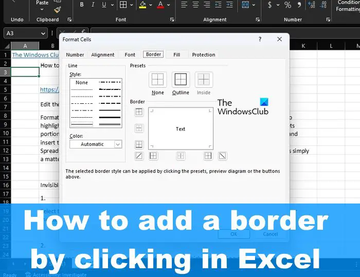
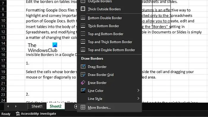
Additionally, if you click on the Border icon once more, you can click on More Borders for advanced options.
I hope this explains how you can add a Border to one or more Cells in Excel.
Read: How to remove Spaces between Characters and Numbers in Excel?
How to put border lines around each cell in Excel?
To put the border line around each cell in Excel, you must first open a sheet, then select the relevant cell or cells. Click on the down arrow button that sits close to the Borders button. Choose the Thick Box Border option to insert a border around the selected cells.
How do I automatically add a border in Excel?
Go to the Border section and select the preferred style of color relating to the lines of the Line fame. After that, be sure to click Outlook via the Presents menu, and ensure that you’re able to see a preview of the lines located in the Border frame. A gridline in the color red is placed on each cell. Finally, hit the IK button and return to the worksheet from whence you came.
Leave a Reply