If you want to add parentheses in Excel, here is how you can do that. Although the manual method works pretty well when you want to add round brackets around one or two cells, you can use this guide to do the same thing to multiple texts at once.

Let’s assume that you have some phone numbers with country codes, and you want to separate them so that other users can recognize them quickly or do not face problems identifying them. The most suitable method is using parentheses, which look like “().” Or, let’s say that you have a few names or any other texts, and you want to add brackets around them. You can go through this guide to get the job done in such situations.
There are two main methods – you can use the Replace option or a Formula. Here, we have discussed both, along with the pros and cons. You can use them as per your requirements.
How to add parentheses in Excel using Replace option
To add parentheses in Excel using Replace option, follow these steps:
- Open the Excel spreadsheet.
- Click on the Find & Select button.
- Choose the Replace option.
- Enter the name/number in the Find what box.
- Enter the same name/number like this: (name/number).
- Click the Replace All button.
To learn more about these steps, continue reading.
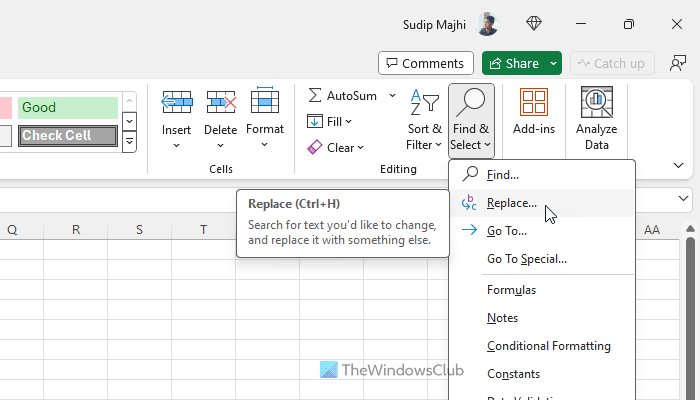
To get started, you need to open the Excel spreadsheet and head to the Editing section in the Home tab. Then, click on the Find & Select button and choose the Replace option.

Alternatively, you can press Ctrl+H to open the same panel. Once it appears, you need to click on the Find what box and enter the text or number.
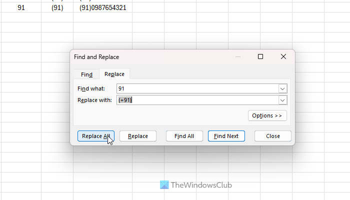
Then, click on the Replace with box and enter the same thing with parentheses. That said, if there is a number called 910987654321 and you want to add parentheses around 91, you need to enter 91 in the Find what box and (91) in the Replace with box.

Finally, click on the Replace All button.
Although this process looks smooth, there is a disadvantage to using this method. As you have seen, it replaces all the numbers or texts at once; if the same thing or combination of numbers is there in the middle or end of the cell, it will replace them as well.
To be more specific, let’s say that you have a number called 9109876549132. If you use the Find and Replace tool, it will look like this: (91) 0987654(91)32. That is why we have tried another method, and it is by using a formula.
How to add parentheses in Excel
To add parentheses in Excel, follow these steps:
- Open the Excel spreadsheet on your PC.
- Select a column where you want to extract the text/digits.
- Enter this function: =LEFT(cell-number,[digit])
- Select another column and enter this function: =”(“&cell-number&”)”
- Select another column and enter this function: =REPLACE(original-cell-number,1,2,”parentheses-added-cell”)
First, you need to open the spreadsheet and select a column where you want to extract the first two digits. Then, enter this function:
=LEFT(cell-number,[digit])
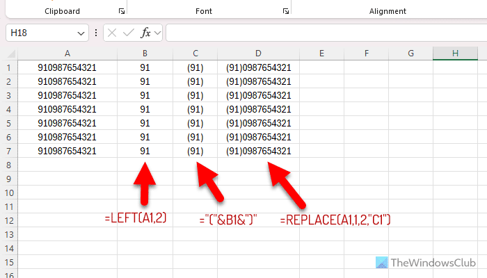
Let’s say you want to extract the first two digits of the A1 cell. If so, enter this function:
=LEFT(A1,2)
Then, select the entire column of extracted numbers and press Ctrl+C to copy. Once done, keep the same column selected and press Ctrl+Shift+V. Following that, choose any cell, click on the exclamatory sign, and click on the Convert to Number option.
Once you do that, your column will remove the function, and you can use the extracted number as an individual cell.
Then, you need to add parentheses by using this formula:
="("&cell-number&")"
If you have extracted the first two digits in column B, you can enter the function like this:
="("&B1&")"
Now, you need to replace the original text with parentheses. For that, use this function:
=REPLACE(original-cell-number,1,2,"parentheses-added-cell")
Keeping the above-mentioned example in mind, you need to enter the function like this:
=REPLACE(A1,1,2,"C1")

Having said that, this function will replace the A1 cell’s first two digits with the C1 cell. If you have tried this with four of five characters, you need to change the 2 in the function with that specific number of characters.
Note: If you want to add the brackets to the entire cell, you do not need to do any of that. You can simply use this formula:
="("&cell-number&")"
That’s all! I hope it helped.
Read: How to use the IMPRODUCT function in Excel
How do you add parentheses in Excel?
To add parentheses in Excel, you can use this function: =” (“&cell-number&”)”. However, here, we have shown several conditional ways to use the same function so that you can replace a certain text with parentheses. There are two main ways to do that, and we have discussed both of them.
How do you insert parentheses in Excel without a formula?
To insert parentheses in Excel without a formula, you can use the Find and Replace panel. Press Ctrl+H to open the panel and enter the original text in the Find what box. Then, enter the same text with parentheses in the Replace with box and click on the Replace All button.
Leave a Reply