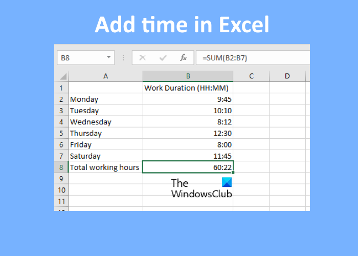
There are some situations when you need to sum up the time in Excel. Let’s say, you have worked on a particular project at different time intervals for a week. To calculate your wages, you need to add the time for all 7 days. You can do it manually on pen and paper but Microsoft Excel makes it easier for you. In this article, we will show you how to add Time in Microsoft Excel.
How to add or sum the Time in Microsoft Excel
Here, we will describe the following two cases:
- When the sum is less than 24 hours.
- When the sum exceeds 24 hours.
1] When the sum is less than 24 hours
Let’s see how to add time in Excel when the total value of the data is less than 24 hours. Follow the instructions listed below:
- Launch Microsoft Excel.
- Enter the summation formula by using the Autosum function for the selected cells.
- Press Enter.
Let’s see these steps in detail.
1] Launch Microsoft Excel and open your spreadsheet in it. In this tutorial, we have taken sample data.
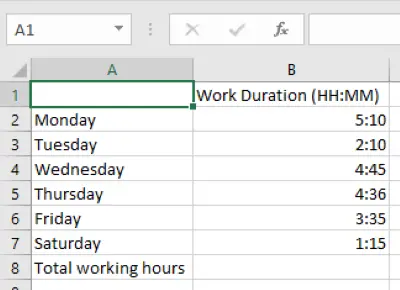
2] Now, select the cell in which you want to display the added time. Type the following formula and press Enter.
=SUM(B2:B7)
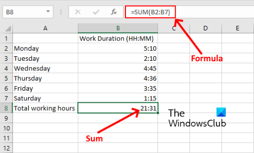
In the above summation formula, B2:B7 indicates that we want to add all the values from cell B2 to B7. Hence, you have to enter the formula as per the data in your Excel sheet.
Read: How to switch Rows and Columns in Excel.
2] When the sum exceeds 24 hours
In the above example, we have taken the data, in which the summation of time is less than 24 hours. Now, we will take another sample data, in which the summation of time exceeds 24 hours. There is no change in the summation formula. What you have to do is format the cell.
Follow the below-listed steps:
- Launch Microsoft Excel.
- Select the cell in which you want to display the sum of time and use the Autosum function.
- Press Enter.
- Format the cell.
Let’s see these steps in detail:
1] Launch Microsoft Excel and open your spreadsheet in it.
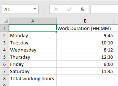
2] Now, select the cell in which you want to display the added time and enter the following formula.
=SUM(B2:B7)
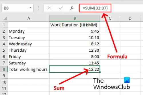
In the above formula, you have to replace B2:B7 with the cells as per your data in the spreadsheet.
3] As you can see in the above screenshot, we do not get an accurate result. Hence, we need to format the cell to display the correct sum of time. To do so, first, select the cell, then go to “Home > Format > Format Cells.” Alternatively, you can right-click on the selected cell and click Format Cells. This will open a new window.
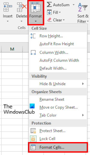
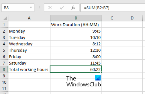
4] Now, select the Custom option in the Category box and then select [h]:mm:ss in the Type box. After that click OK to save the settings. This will display the accurate sum of time.
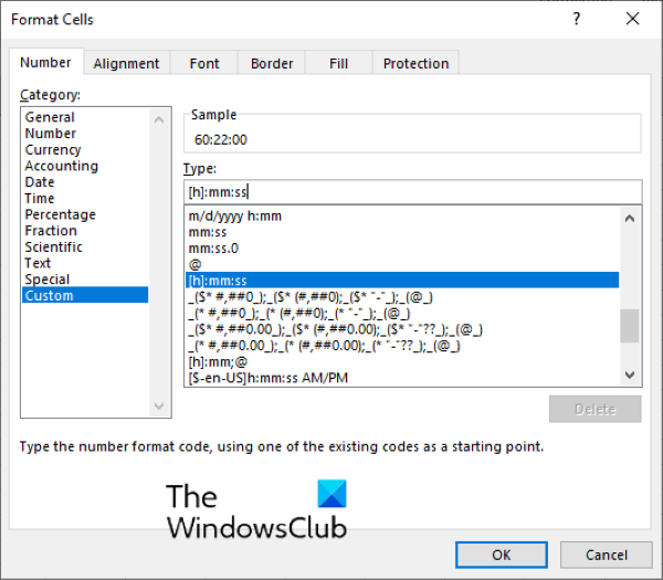
The custom format that we have selected displays the time in HH:MM:SS format. If you do not want to display the seconds, delete ss from the format [h]:mm:ss.
That’s it.
Related posts:
Leave a Reply