GPA or Grade Point Average is an important parameter used to judge the average results of students in most universities in Western countries, especially the USA. The GPA helps companies understand the overall result of a student over a short scale (usually 0 to 5). If you wish to calculate GPA in Excel, please read this article.
How to calculate GPA in Excel
GPA doesn’t have a fixed scale and usually varies across universities. So, we will create a scale table in Excel to decide the parameters and then use it in an example. We will need three parameters to find the GPA: percentage, grade, and grade value.
Note: This procedure works with the MS Excel for Windows version and not the web version.
Let us assume the grade process as follows:
0% to 39% = F grade or 0 value
40% to 49% = D grade or 1 value
50% to 59% = C grade or 2 value
60% to 79% = B grade or 3 value
80% and above = A grade or 4 value
The formula for GPA is as follows:
GPA = Sum of grade values in all subjects / Total number of subjects
The Excel formula for GPA becomes:
=<cell with sum of grade values>/<total number of subjects>
This could be better understood through an example.
Eg. Let us assume the following example. Proceed step by step to find the GPA.
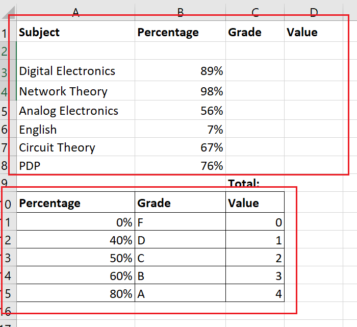
1] The percentages scored by a student in various subjects are in columns A and B, the grades need to be mentioned in column C, and the grade values in column D as shown in the picture below.

2] Create a second table with fixed values for judging the grade and value as per percentage scored. The percentage should be the least needed to score a certain grade. Create borders for this second table to distinguish it from the first one.
3] Click on the cell in which you need the first-grade value once (double-click will enable text so don’t do that).
4] Go to Formulas > Lookup & Reference.
5] Select VLOOKUP from the list of functions. This would open the Function arguments window.
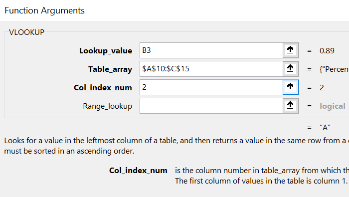
6] In the Lookup_value field, type the cell coordinates of the first cell with the percentage scored.
7] For Table_Array, select the second table which you would use for reference values. Then, add $ before and after each column letter. In my case, the formula for the table array becomes $A$10:$C$15.
8] In the Col_index_num, mention the column number in the selected table. In my case, since I need the grade and the grade reference is in the second column, the Col_index_num becomes 2.

9] Hit Ok. You would get the grade corresponding to the percentage in the selected cell (in my case C3).
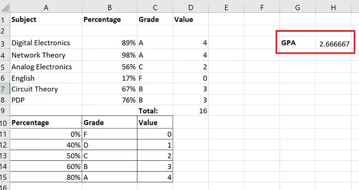
10] Use the Fill function to pull the results down to the last row with the percentage. To do so, click outside cell C3 and then back on it. Then, use the little dot at the right-bottom corner of the selected cell C3 to pull the formula down to cell C8.
11] To find the list of values, use the same procedure you used for the grade, with the difference that the Col_index_num would be 3.
12] Use AutoSum to find the sum of all grade values in cell D9.
13] To find the GPA in cell H3, the formula becomes:
=D9/6
14] Hit Enter.

There you have it!
Please let us know in the comment section if you have any doubts about the procedure.
I hope this was helpful.
Read: Merge and Center button is missing, grayed out or not working in Excel.
How to calculate average GPA in Excel?
You need to use this formula to calculate the average GPA in Excel: =<cell with sum of grade values>/<total number of subjects>. Then, you can use VLOOKUP to enter the grades. You need to enter the Lookup_value, Table_array, Col_index_num, etc., as per the data you want to calculate.
How do you calculate average and grade in Excel?
To calculate the average, you need to divide the total grade by the total number of subjects. On the other hand, to calculate grades, you need to choose the values first. For that, you can use the VLOOKUP.
Read: How to calculate the area of a Rectangle, Triangle or Circle in Excel.
Leave a Reply