In this post, we will show you how to change the Gridline color in Excel. Gridlines are the lightly visible lines that appear around cells in a worksheet to differentiate them and make the data easier to read and organize. By default, they’re light grey in color. However, if you wish, you can change the color of your gridlines in many different ways.

How to change Gridline color in Excel
The following methods let you change the Gridline color in an Excel worksheet on a Windows 11/10 PC:
- Excel Options
- Cell Borders
- Line Color
- Conditional Formatting
- VBA
Let us see this in detail.
1] Excel Options
In Excel, there’s a direct option to have a different gridline color in your Excel worksheets. To set this color:
Go to File > More… > Options. Switch to the Advanced tab in the Excel Options window and scroll down until you find the Display options for this worksheet section.
At the bottom of this section, click the Gridline color dropdown. Select the desired color from the color palette and click the OK button in the Excel Options window.
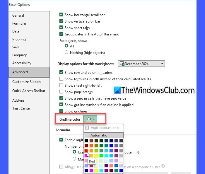
The above steps will change the gridline color of your active worksheet. To change the gridline color of all worksheets, select them by clicking on their respective tabs while holding the Ctrl key. This will group the worksheets (a ‘[Group]’ label will append the workbook’s title on top). After this, when you change the gridline color, it will be applied to all the selected worksheets.
Once you’ve applied a different color to the selected worksheets, don’t forget to ungroup them (right-click the tab and select Ungroup Sheets). If you don’t ungroup the sheets, further changes in your active worksheets will be applied to the rest of the sheets as well.
Note: Changing the gridline color won’t affect the default color (light grey) of the new worksheet(s)/workbook(s).
2] Cell Borders
Border and gridlines are different in Excel. Gridlines appear on the entire worksheet by default, while borders can be applied manually around a cell or a range of cells to highlight the data.
You can mimic a change in gridline color by applying borders to the cells in the desired shade. Here’s how:
Select the cell or the cell range, click the Borders dropdown in the Home menu (under Font), and select More Borders. This will bring the Format Cells dialogue with the ‘Border’ tab selected by default. Click the Color dropdown on the left side and select the color you want to apply to the gridlines. Next, click the Outline and Inside preview options on the right side. You’ll see the changes in the diagram shown below the options. Click OK to apply the borders.
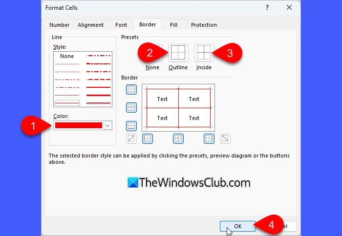
The above steps override the default gridlines and create visible, colored borders around the selected cell(s).
3] Line Color
Line Color is part of the Borders feature. It can be useful if you want to emphasize specific cells with colored borders instead of relying on the default gridlines.
To change the Line Color in Excel, click the dropdown next to the Borders icon and hover over Line Color. Select the desired color from the color palette.
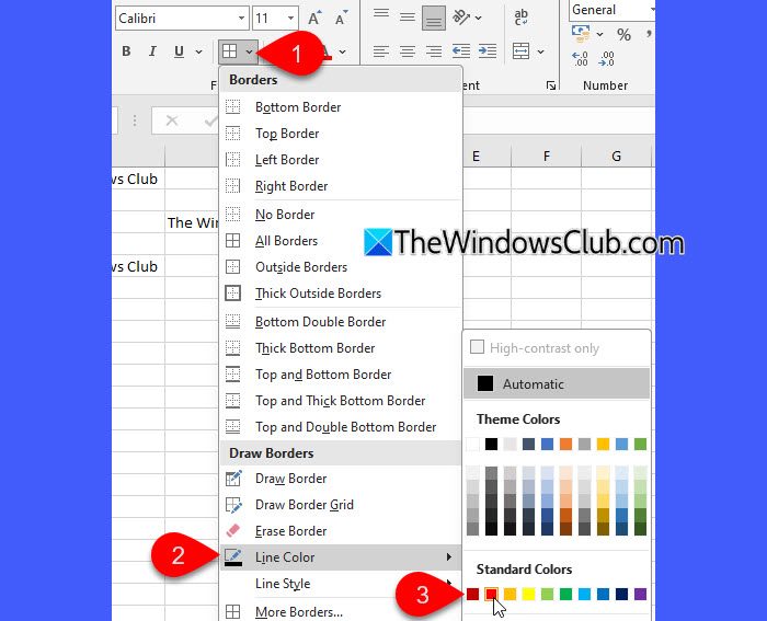
Your mouse pointer will turn into a pencil icon. Move the pencil over the cell border where you want to apply the color and click to apply it.

4] Conditional Formatting
Condition Formatting visually mimics gridline color changes but applies only to selected areas (based on the set condition).
Select the cell(s) where you want custom gridlines or the entire worksheet. Click the Conditional Formatting dropdown in the Home menu and select New Rule.
In the New Formatting Rule dialogue, select a Rule Type. For example, if you want to change the gridline color for cells that contain a specific value/text, select Format only cells that contain, then under the Edit Rule Description, select Cell Value > equal to > [value/text].
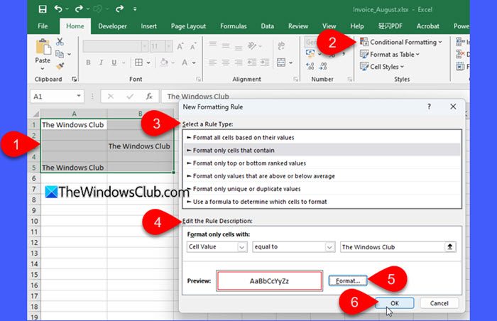
Next, click the Format button to select a border color and preset (as explained above). Click OK to apply the rule.
5] VBA
Advanced users may use VBA to change the gridline color in Excel. Here’s how:
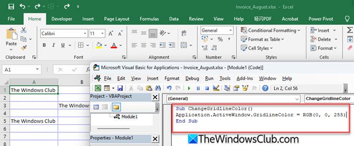
Press Alt + F11 to open the VBA editor. Click Insert > Module, and paste the following code in the code editor window:
Sub ChangeGridlineColor()
Application.ActiveWindow.GridlineColor = RGB([RedValue], [GreenValue], [BlueValue])
End Sub
Replace [RedValue], [GreenValue], and [BlueValue] with values between 0 and 255 for each color channel. For example, enter RGB(0, 0, 255) for Blue color. Run the macro to update gridline colors.
To change the gridline color back to default, go to File > Options > Advanced and select Automatic as the Gridline color.
That’s all! I hope you find this useful.
Read: How to change Gridline style and background color in Access datasheet.
How do I customize the grid in Excel?
To customize the gridlines in your Excel worksheet, you can change their color, apply borders to them, or apply a fill color to selected cells. If you do not want the gridlines to appear in your worksheets, you may choose to hide them. You may also resize the gridlines by adjusting the row height or column width in the worksheet (Home > Format > Row Height/Column Width).
How do I color grid lines in Excel?
To apply a custom color to the gridline in your Excel worksheet, click on the File menu and select More > Options. Then go to Advanced > Display options for this worksheet. Click the Gridline color dropdown and choose the desired color. Click OK to save the changes.
Read Next: Excel not printing gridlines properly.
Leave a Reply