Microsoft Excel is well known for creating charts for marketing purposes, and it has features to perform various calculations. Charts are a graphical representation of your data, and they make showing comparisons and trends much easier for your audience to understand. In Excel, users can add predefined layouts and styles to format their charts quickly. In this tutorial, we will explain how to apply layouts and styles to your chart in Microsoft Excel.

How to change Layout and Chart Style in Excel
Follow the steps below to apply layouts and styles to your chart in Excel:
How to change the layout of the Excel chart

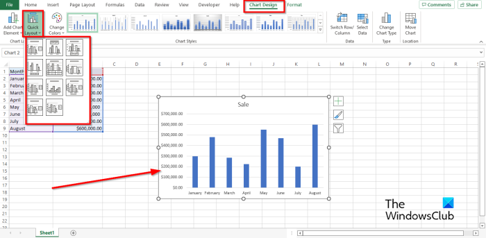
Select the chart, then go on the Chart Design tab and select the Quick Layout button in the Chart Layouts group and select an option from the menu.
In the Quick Layout group, there are 11 layouts, namely:
Layout 1: Layout 1 shows the following elements: Chart Title, Legend (Right), Horizontal Axis, Vertical Axis, and Major Gridlines.
Layout 2: Layout 2 shows the following chart elements: Chart Title, Legend (Top), Data Labels (Outside End), and Horizontal Axis.
Layout 3: Layout 3 shows the following elements: Chart Title, Legend (Bottom), Horizontal axis, Vertical Axis, and Major Gridlines.
Layout 4: Layout 4 shows the following chart elements: Legend (Bottom), Data Labels (Outside End), Horizontal Axis, and Vertical Axis.
Layout 5: Layout 5 shows the following elements: Chart Title, Data Table, Vertical Axis Title, Vertical Axis, and Major Gridlines.
Layout 6: Layout 6 shows the following elements: Chart Title, Vertical Axis Title, Data Labels on Last Category (Outside End), Horizontal axis, Vertical Axis, and Major Gridlines.
Layout 7: Layout 7 shows the following chart elements: Legend (Right), Horizontal Axis Title, Vertical Axis Title, Vertical Axis, Major Gridlines, and Minor Gridlines.
Layout 8: Layout 8 shows the following elements: Chart Title, Horizontal Axis Title, Vertical Axis Title, Horizontal Axis, and Vertical Axis.
Layout 9: Layout 9 shows the following chart elements: Chart Title, Legend (Right), Horizontal Axis Title, Vertical Axis Title, Horizontal Axis, Vertical Axis, and Major Gridlines.
Layout 10: Layout 10 shows the following chart elements: Chart Title, Legend (Right), Data Labels (Outside End), Horizontal Axis, Vertical Axis, and Major Gridlines.
Layout 11: Layout 11 shows the following chart elements: Legend (Right), Horizontal Axis, Vertical Axis, and Major Gridlines.
Any Layout Style you have chosen is how the layout is going to be.
How to apply styles to the chart in Excel

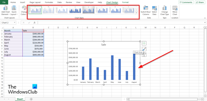
Select the chart and click any of the styles in the Chart Styles gallery on the Chart Design tab.
What is chart style in Excel?
The Chart Style is a feature that lets users customize their charts into different styles offered in the gallery. In Microsoft Excel 365 there is a total of 16 chart styles in the Chart gallery. In this tutorial, we have explained how to add chart styles to Excel.
READ: How to crop an image to shape in Excel
What is chart layout in Excel?
The Chart Layout in Microsoft Excel is a feature that changes the overall layout of the chart design; it showcases information about the design of the structure and the design of the various graphs. It determines how each graph is arranged.
How do I save a chart layout in Excel?
Follow the steps below on how to save a Chart Layout in Microsoft Excel:
- Select the chart, then choose a Chart Layout Style.
- Then right-click the chart with the layout and select Save as Template in the context menu.
- A Save Chart Template dialog box is open.
- Choose the location where you want to save the template, then click Save.
- Now we have a chart template.
How do you edit a chart in Excel?
Follow the steps below to change the Chart Type in Excel:
- Select the Chart, then click the Change Chart Type button in the Type group on the Chart Design tab.
- A Change Chart Type dialog box will open.
- Choose a different Chart, then click OK.
- The Chart Type is changed.
Where is chart Design tab Excel?
The Chart Design tab in Microsoft Excel is only available when a chart is inserted into the spreadsheet and is selected. When the chart is selected, a Chart Design tab will appear on the menu bar. The Chart Design tab consists of features to customize the chart.
READ: How to create a Combination Chart in Microsoft Excel
We hope this tutorial helps you understand how to apply layouts and styles to your chart in Excel.