In this post, we will show you how to change lowercase to uppercase in Excel. Textual data in Excel often consists of datasets that are written in lowercase. Sometimes, we require changing this data to the proper case to make it syntactically correct or to uppercase for specific reasons.
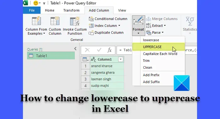
Unfortunately, Excel doesn’t have a built-in option to change the case of the text like other Office tools have (Word and PowerPoint). However, there are ways using which you can easily change the text case in your Excel spreadsheets. In this post, we will look into various methods of changing the text from lowercase to uppercase in Microsoft Excel.
How to change Lowercase to Uppercase in Excel
To change lowercase to uppercase in Excel, you may use the following methods:
- Use the UPPER() function
- Use the Flash Fill feature
- Use Power Query
- Use Power Pivot row-level formula
- Use an All Caps font
Let us have a detailed look at all these methods.
1] Use the UPPER() function
You may use the UPPER() function in Excel to change the case of the text to uppercase. UPPER() is one of many text functions that can transform text in Excel spreadsheets. It has the following syntax:
UPPER(text)
- Where text represents the string that needs to be capitalized.
Let us see how you may use this function to change lowercase to uppercase in Excel. Suppose we have a spreadsheet wherein we have some sample data as shown in the below image.

The above sample data consists of the names of the authors of TheWindowsClub in Column A. As you can see, all the names are written in lowercase. To convert the names in uppercase, you may use the UPPER() function as follows:
Place your cursor in cell B2. Type the following formula in the Formula Bar on top: =UPPER(A2).
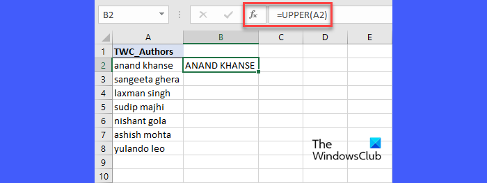
Press the Enter key. This will convert the data in cell A2 in uppercase.
To apply the same formula to all other values in Column B, select cell B2 and take your cursor to the bottom-right corner of the cell. As it turns into a plus (+) symbol, click and drag the cursor till cell B8. Release the mouse button to view the results.
2] Use the Flash Fill feature
Many of us may not know that Excel comes with a Flash Fill feature. This feature automatically fills in values based on a couple of examples provided by the users. If you manually enter the data in uppercase in at least 2 cells, Flash Fill can analyze the pattern and transform the rest of the data for you. Let’s see how.
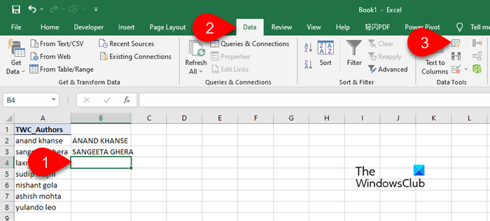
Taking the same example, place your cursor in cell B2 and type ‘ANAND KHANSE’. Then place the cursor in cell B3 and type ‘SANGEETA GHERA’. As you type the second word, Flash Fill will show suggested values in light-grey color to be filled in the rest of the cells.

Press the Tab key to accept the suggestions (press ‘Enter’ to reject).
The Flash Fill feature works only to the right of the data that needs to be transformed. You can also access Flash Fill from the Data tab.
Place your cursor in cell B4 (after inputting values in cells B2 and B3 ) and click on the Flash Fill icon under Data Tools.
Alternatively, you may use the Ctrl+E hotkey to activate Flash Fill.
3] Use Power Query
Power Query, also known as ‘Get & Transform’ in Excel, is all about transforming or reshaping data. You can use it to easily convert your lowercase data to uppercase in an Excel spreadsheet. Here’s how:
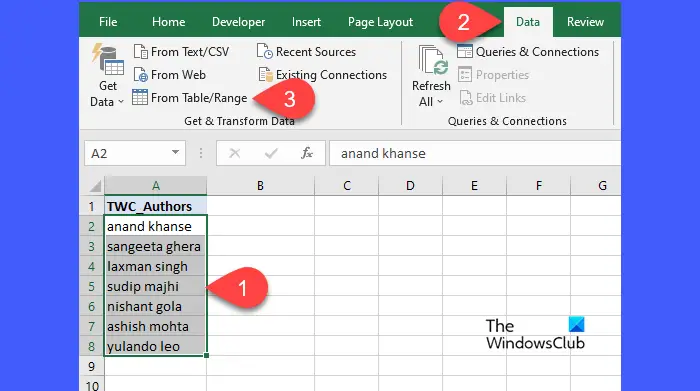
Select the cell range that contains the actual data (A2:A8). Go to the Data tab. Click on the From Table/Range option under the Get & Transform Data section.
Click OK in the Create Table popup. Power Query Editor will open up.
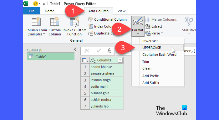
Switch to the Add Column tab. Select Format > UPPERCASE under the From Text section.
Switch to the Home tab.
Click on the Close & Load option in the top left corner.
A table consisting of two columns will appear in a separate spreadsheet. The second column will display data in uppercase. You can copy these column values and paste the data into your main spreadsheet (over the lowercase values). After that, you can delete the new spreadsheet and keep the main spreadsheet in your Excel file.
Read: Microsoft Power Query for Excel helps with data discovery.
4] Use Power Pivot row-level formula
This method uses the Power Pivot add-in, which allows you to create pivot tables by linking columns from different tables. Using this add-in, you can perform row-level calculations and add new calculated columns to your main data. These calculations/formulas work similarly to the regular Excel functions.
Power Pivot is not available in all versions of Excel. Visit this link to check if your version of Excel/Office includes Power Pivot. If it does, you need to enable it first, as it is not enabled by default.
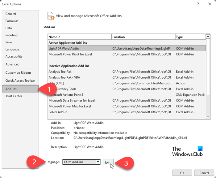
To enable the Power Pivot add-in, go to File > More… > Options. Select the Add-ins tab in the Excel Options window. Select COM Add-ins in Manage dropdown at the bottom. Click on the Go… button.
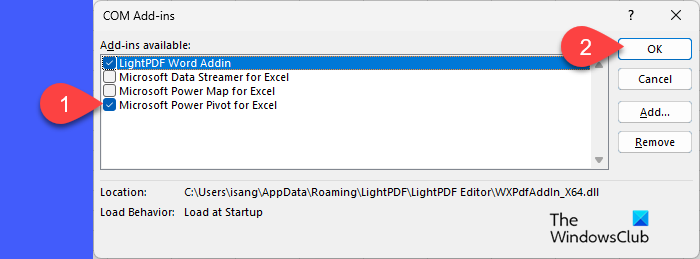
Tick the checkbox for Microsoft Power Pivot for Excel in the COM Add-ins window. Click on the OK button.
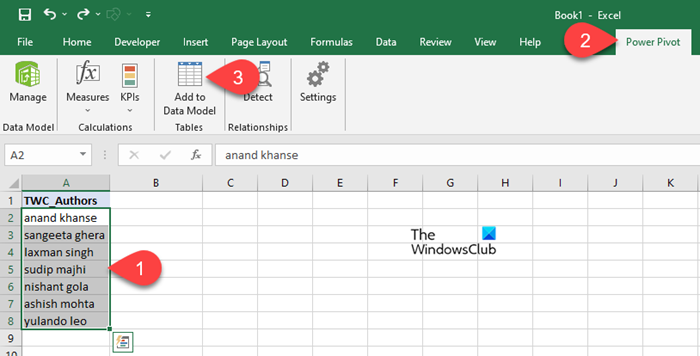
The Power Pivot tab will appear in your Excel program window. Now you may use it to change lowercase to uppercase in Excel. Here’s how:
Select the cell range that contains the data in lowercase (A2:A8). Go to the Power Pivot tab. Click on the Add to Data Model option.
Click OK in the Create Table popup. In the Power Pivot for Excel window, place your cursor in an empty cell in the column labeled Add Column. Enter the following formula in the Formula Bar on top: =UPPER([TWC_Authors].
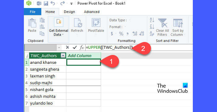
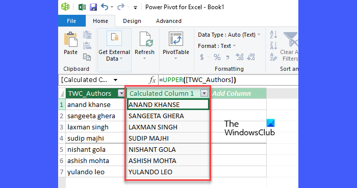
Press the Enter key. A ‘calculated column’ will appear. Each row in the calculated column uses the same formula that has been applied to the selected cell. So you’ll get row-level results using a single formula.
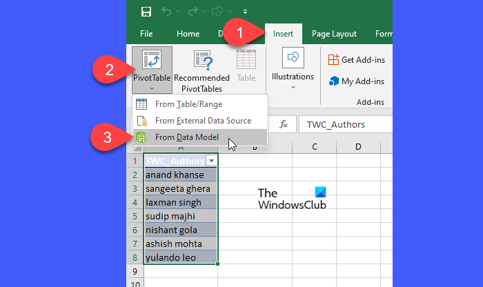
Close the Power Pivot window. Go to the Insert tab in your main Excel window. Select Pivot Table > From Data Model.
In the PivotTable from Data Model popup, select New Worksheet and click on the OK button.
Expand the Data Source Table in the PivotTable Fields panel on the right. Select Calculated Column. Column values will appear in the spreadsheet.
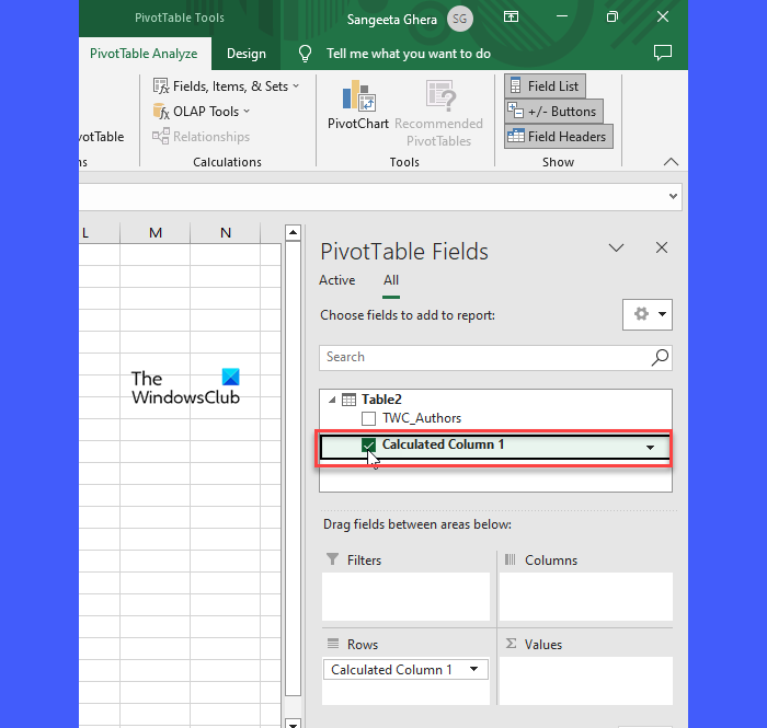
Copy the uppercase values from this new spreadsheet and paste the data over the lowercase values in the main spreadsheet.
Note: All the methods discussed so far produce results in a different column. So you need to delete the original column (with lowercase values) and keep the new column (with uppercase values) after renaming the header (if any), or copy-paste data from one spreadsheet to the other. However, if you want to change the case of the text in the original column itself, you can use the next method.
5] Use an All Caps font
If there isn’t any specific font to display the data in your Excel spreadsheet, you may change lowercase to uppercase using an All Caps font, such as Algerian, Copperplate Gothic, and Engravers MT. These fonts always use the uppercase versions of the letters, so it won’t matter whether the text is written in uppercase or lowercase – these are ideal to replace the lowercase letters with large caps within the existing column.
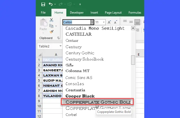
- Select the data range that needs to be transformed (A2:A8)
- Go to the Home tab.
- Click on the Font dropdown and select an All Caps font. You will see the changes in real time.
This is how you change lowercase to uppercase in Microsoft Excel.
I hope you find this useful.
Also Read: How to change the Case of Text in Word and Google Docs.
What is the shortcut key for change case in Excel?
There’s no hotkey or keyboard shortcut for changing the text case in Excel since ‘Change case’ is not a built-in feature in Excel. However, you can use Excel functions to change the case of a given text or string value. The UPPER() function transforms a given text to uppercase, the LOWER() function transforms it to lowercase, and the PROPER() function transforms it to proper case.
How to change lowercase to uppercase in Excel without formula?
You can use the Flash Fill feature to change the case of text in Excel without using the UPPER() function. You just need to enter the first few values. Flash Fill will quickly analyze your pattern and suggest further values to be auto-filled in the rest of the cells. Apart from this, you can use Power Query or an All Caps font.
Read Next: How to Mail Merge from Excel to Outlook.