Comparing two columns in Excel doesn’t have to be a difficult task, and to get the job done, we suggest using VLOOKUP. You see, not always; the columns you want to compare are in the same workbook or spreadsheet; therefore, the traditional way of comparing things would increase the workload. This tutorial will explain how to use the VLOOKUP formula to compare a maximum of two columns in a bid to have common values returned or to locate missing data.

How to compare columns in Microsoft Excel
As stated, we can use the Excel VLOOKUP function to find and match different data or find differences in two columns.
- Compare columns (Find and match different data)
- Find differences by comparing two columns
1] Compare columns (Find and match different data)

In many cases, you will likely have two columns in an Excel spreadsheet with data, and your task is to find out whether or not a data point in one of the cells exists. A situation like this does not require the use of the IF function or the equal-to sign, but rather VLOOKUP.
Let us explain how to get the job done in record time and without issues.
Launch the Microsoft Excel application.
After that, please open a workbook or spreadsheet that contains the data.
If you’ve yet to add data, then please open a new spreadsheet, then populate it with relevant information.
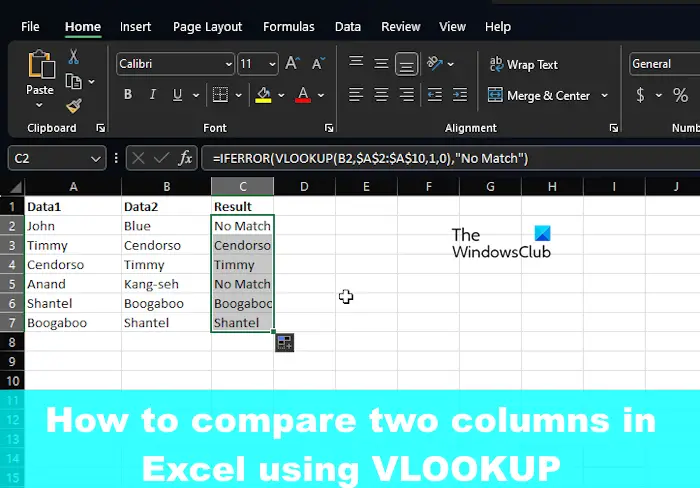
Now, if you have a dataset where both column A and column B are populated with names, you can have the same names from both columns show up in column C. For example, if Myrtle is situated in both A and B, then VLOOKUP can place that name in C.
All you have to do is type the following command:
=IFERROR(VLOOKUP(B2,$A$2:$A$10,1,0),"No Match")
Bear in mind we use No Match for whenever a match is not found. In that case, the words No Match will appear instead of a blank space or #N/A.
2] Find differences by comparing two columns

Another purpose for the VLOOKUP function is to find differences within two columns. This is an easy task, so let us talk about how to get this done.
We suspect you already have Excel up and running along with the workbook with all the data.
So, we suspect that you have data in columns A and B, for example, names.
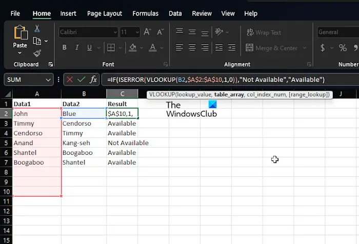
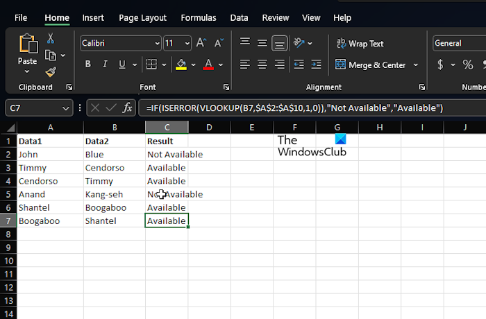
If you need to find out the names that are located in Column B that are not available in Column A, then use the following command:
=IF(ISERROR(VLOOKUP(B2,$A$2:$A$10,1,0)),"Not Available","Available")
The formula above will check the name in column B against all names in column A. If it finds an exact match, the formula will ensure the name is returned, and if not, #N/A will appear instead. Because of this, we chose to include IF and ISERROR functions wrapped up with VLOOKUP.
So, when the name is missing, this formula will showcase Not Available, and if present, it will return Available.
READ: Fix Excel found unreadable content error
Can VLOOKUP return 2 columns?
If you want to VLOOKUP more than one column at once, simply create one array formula or use helper columns if you’re not interested in using array formulas.
What is the VLOOKUP formula example?
Use the VLOOKUP formula in Excel to find values in a table. For example, you can use =VLOOKUP(A2,A10:C20,2,TRUE) or =VLOOKUP("Fontana",B2:E7,2,FALSE) as an alternative. It is all based on the columns and what you want to achieve.
Leave a Reply