Sometimes, we need to sort data in Excel based on the number of occurrences of a text. In this case, if we count the occurrences manually, it will take more time. Moreover, if we have a huge dataset in Excel, calculating the occurrences of a text is almost impossible. In this article, we will show you an easy way to count the frequency of a text in Excel.

How to count the frequency of a text in Excel
To count the frequency of a text in Excel, you can use the Countif function. We have described the entire process in detail.

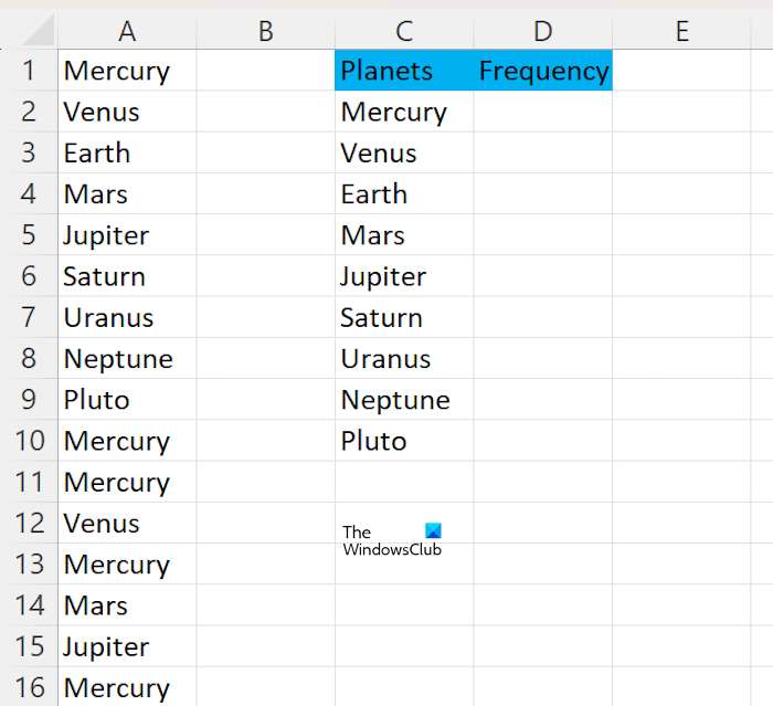
We have created sample data with the names of the planets in Excel (as shown in the above image). Here, we will count the frequency of each planet by using the Countif function.
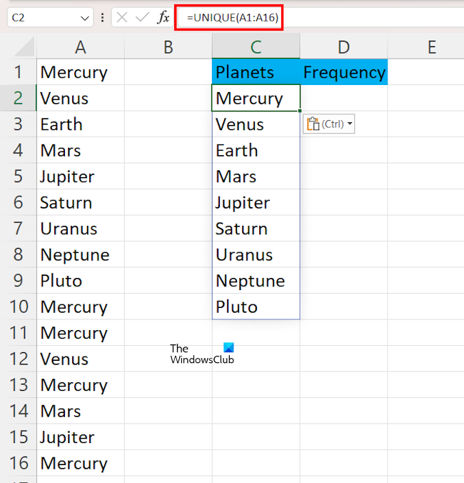
Before applying the Countif function, write all the names in a separate column. You can do this manually. However, if the data is large, doing this manually will consume a lot of time. Therefore, you can use the Unique function. The Unique function creates a list of unique values from the selected range of cells.
To use the Unique function, write the formula written below:
=unique(cell range)

In the above formula, select the right cell range. For example, in our case, the cell range is from A1 to A16; hence, the formula will become:
=unique(A1:A16)
Press Enter after typing the above formula. Now, the next step is to count the frequency of each text. Use the following formula:
=countif(cell range, "criteria")

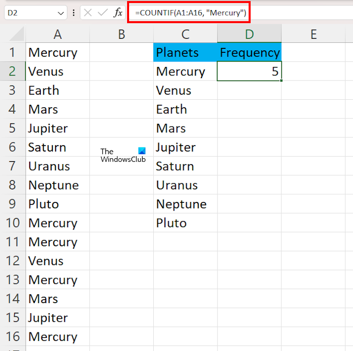
In the above formula, cell range indicates the range of the cells and criteria indicates the text, the frequency of which is to be calculated. For example, in our case, the formula to count the frequency of Mercury is:
=countif(A1:A16, "Mercury")
You have to enter the above formula manually in each cell to count the frequency of different texts. For example, to count the frequency of Venus, the formula will be:
=countif(A1:A16, "Venus")
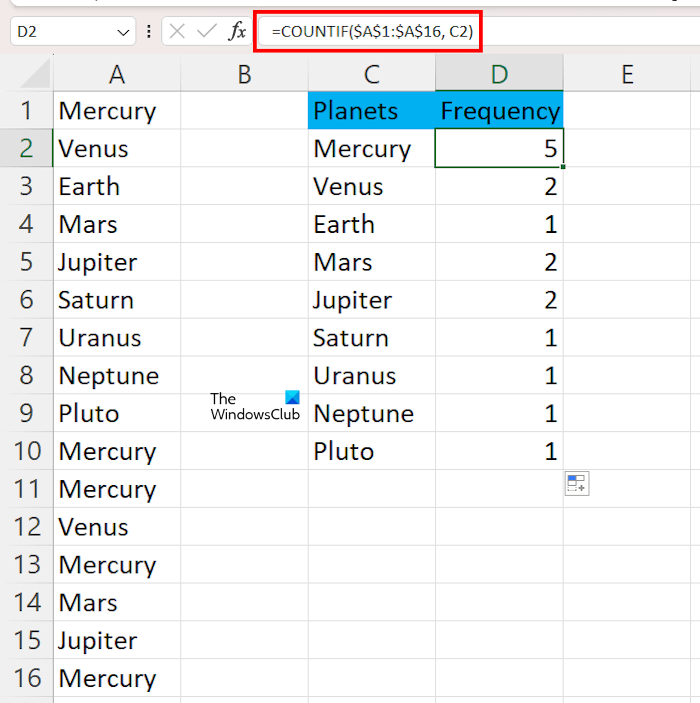
This is a disadvantage, especially when the data is large. This is because it prevents us from using the Fill Handle. To eliminate this disadvantage, lock the cell range and use the cell address in place of values. Locking the cell range is important because if you do not lock the cell range, you will get incorrect values when you apply the same formula to the remaining cells using the Fill Handle.

For example, to calculate the frequency of Mercury, the formula will become:
=COUNTIF($A$1:$A$16, C2)
In the above formula, we have locked the cell range and entered C2, the cell address of Mercury. Now, when you drag the formula to the other cells by using the Fill Handle, it will not show you the incorrect values or errors. You will get the right values.
That’s it. I hope this helps.
How do I find frequent text in Excel?
To find the frequently occurring text in Excel, you can use the following formula:
=INDEX(range, MODE(MATCH(range, range, 0 )))
Enter the same cell range in all places in the above formula.
How to use SUMIF?
The purpose of the SUMIF function is to sum the values in a range that meets the criteria you specify. The formula to use the SUMIF function in Excel is as follows:
SUMIF (range, criteria, [sum_range])
Read next: How to use AVERAGEIF and AVERAGEIFS in Excel.
Leave a Reply