If you want to create a Heatmap in Excel, here is how to do that. It is possible to add colors based on a range of values so that it looks like a heatmap. For that, you do not need any third-party add-in since Excel allows users to make a heatmap using in-built options.
Let’s say that you have a mark sheet of fifty students, and you want to categorize them into three different groups based on the numbers obtained by them. There are mainly two ways to do that. First, you can sort them in descending or ascending order. Second, you can use a heatmap to identify the categories. If you want to use the second method, here is how it can be done.
How to create a Heatmap in Excel
To create a Heatmap in Excel, follow these steps:
- Open the Excel spreadsheet on your computer.
- Select the numbers.
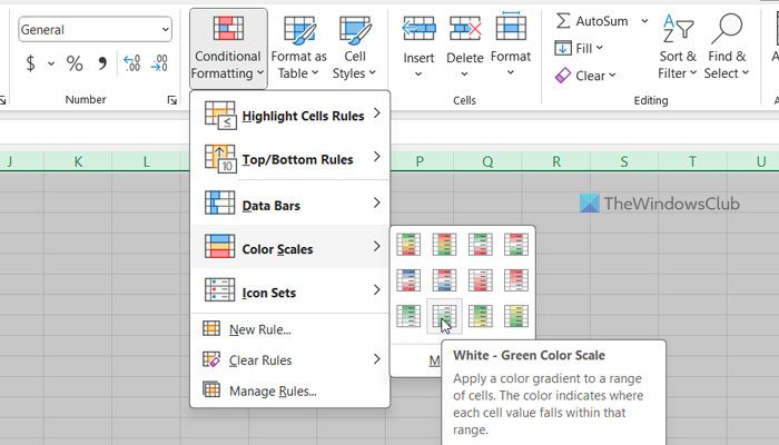
- Click on the Conditional Formatting menu.
- Choose the Color Scales option.
- Select a color scale.
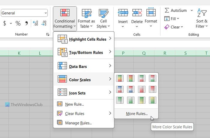
- Click on the More Rules option.
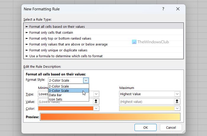
- Select the 3-Color Scale option from the Format Style menu.
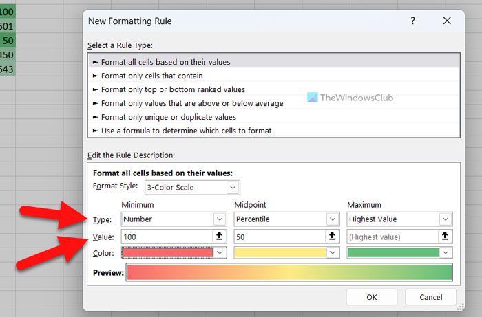
- Expand the Minimum drop-down list and choose Number.
- Enter the lower number.
- Do the same with Midpoint and Maximum.
- Choose the color as per your requirements.
- Click the OK button.
To start, you need to open the Excel spreadsheet and select the numbers. You can select the entire spreadsheet at once as well. Then, click on the Conditional Formatting menu and select the Color Scales option.

Next, you can select a color scale as per your requirements.
Once done, all the numbers will be colored at once automatically. However, if you want to choose custom values and colors, you need to click on the Conditional Formatting > Color Scales > More Rules option.

Ensure that the Format all cells based on their values option is selected. If so, expand the Format Style drop-down menu and choose the 3-Color Scale option.

Next, expand the Minimum drop-down menu and select the Number option. Then, enter a number that you want to set as the minimum value.

Once done, click on the Color menu and choose a color as per your requirements.
Following that, do the same with Midpoint and Maximum.
Finally, click the OK button.
That’s all! Hope this guide helped you.
Read: How to create a Chart with Crayon effect in Excel
How do I create a heatmap chart in Excel?
To create a heatmap chart in Excel, you need to use the Color Scales option. For that, select the list of numbers and choose the Color Scales option from the Conditional Formatting menu. However, you can also create a custom rule to format the numbers as per your requirements. In that case, you can choose the minimum, midpoint, and maximum values accordingly.
Can Excel generate a heat map?
Yes, Excel can generate a heatmap. Although it cannot do that on its own, you can create it manually. For that, you need to use the Color Scales option, which is available under the Conditional Formatting. It is also possible to create a custom rule and customize the heatmap with different conditions.
Read: How to change default Chart Color in Word, Excel, PowerPoint
Leave a Reply