Excel users who regularly reference the same cell in ranges from within their Workbook, will be happy to know that the popular platform has an easier way to create a named range. It is considered the best way to reference a cell range. In this post, we will show yo how to create Named Ranges in Excel.

Here is an example. If you have key sales data in cells D3:D16 that you refer to constantly, you could make the decision to create a named range called MonthlySales and use it instead of the D3:D16 cell range.
How to create Named Ranges in Excel
To name a range in Microsoft Excel, you can use any one of these methods.
Name a range using the Formulas tab in Excel

Naming a range from the Formulas tab is one of the best ways to get the job done, so if you’re not sure how, well, let us take the time to explain.
- First, you must open Excel and the Workbook you wish to edit.
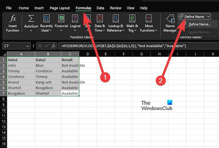
- Select the cells you wish to include in your named range.
- From here, click on the Formulas tab on the Ribbon, then select Define Name.
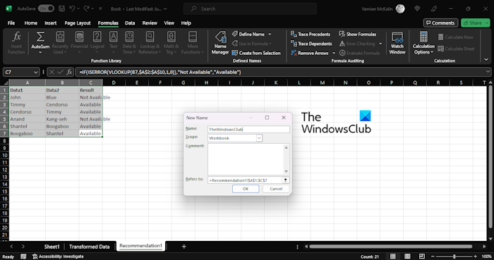
- Type a name for your named range in the Name box.
- When it comes down to Scope, just leave it as Workbook and do not change it.
- If you feel the need, go ahead and leave a description in the optional Comment field.
- When it comes down to the Refers to field, this should be pre-filled with the selected cells.

Click the OK button to close and return to the Excel sheet.
READ: How to enable and use VBA in Excel
Name ranges from the Name box in Excel

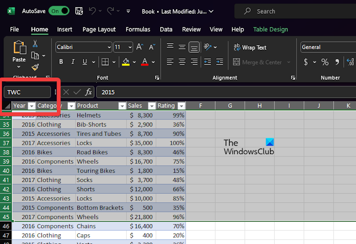
One of the easiest ways to name a range is with the name box feature. You can find it on the left side below the Ribbon.
The name box usually showcases the name of the cell or range you’ve selected. Additionally, it can also be used to name ranges and cells with ease.
Let us explain how to take advantage of this important Microsoft Excel feature.
- Open the Excel application.
- Create a new Workbook or open one that was created prior.
- From here, choose the range or cell you want to give a name to.
- The next step is to type the preferred name directly into the name box.
- Complete the task by pressing the Enter key to create a named range.
READ: Fix Excel found unreadable content error
Name a range from the Name Manager in Excel
For those who are wondering, the Name Manager is the consolidated location where all your named ranges are found. So, let us look at how to use the Name Manager to create a named range.
- We suspect Excel is up and running, and the relevant chart opened.
- From the chart, click on the Formulas tab, then select Name Manager from the Ribbon.
- You now only need to follow the steps from the first solution to define your named range via the New Name window.
READ: How to calculate ratio in Excel
Use a keyboard shortcut to create Named Ranges in Excel
Finally, we want to look at how to use a keyboard shortcut to name ranges in Microsoft Excel. This is for those who live by using the keyboard rather than anything else since the steps are faster.
- Begin by pressing CTRL + F3 from your Workbook to open the Name Manager.
- After that, press CTRL + SHIFT + F3 to open the Create From Selection area.
- Type in the relevant details, and that’s it for that, you’re done.
READ: How to compare two columns in Excel using VLOOKUP
How do I create a range table in Excel?
The first thing to do is select a cell within your data. From there, click on Home > Format as Table, then choose a style for the table. From within the Create Table dialog box, please set your cell range. Finally, mark if your table has headers, then hit the OK button.
Read: How to count number of comma-separated values in a single cell
Why Use Named Ranges?
The reason to use named ranges is to ensure that your Excel calculations are more understandable to yourself and others. For example, a formula that contains a named range such as =SUM(MonthlySales) gives a better indication of the overall calculation when compared to =SUM(C3:C14). Additionally, a named range is easier to update if the underlying cell range changes. Always remember this when deciding which option to choose.
Leave a Reply