Finding percentage change in Excel requires calculating the difference between two numbers, dividing that difference by the successive number and changing the decimal value to a percentage. In case of a range of numbers, you could pull the formula down across the range of numbers.
How do you calculate percentage increase or decrease in Excel
Let us understand the basics of the percentage change. The percentage change is (new value-old value)/old value. Thus, the syntax for the percentage change formula becomes:
=(<cell with new value>-<cell with old value>)/<cell with old value>
Where,
- <cell with new value> is the second cell in the calculation
- <cell with old value> is the first cell in the calculation
This formula could be applicable for any two random cells across the Excel sheet, except when you need to find the results across a range of cells using the Fill option. In that case, the cells in discussion need to be placed in the same row across two different columns.
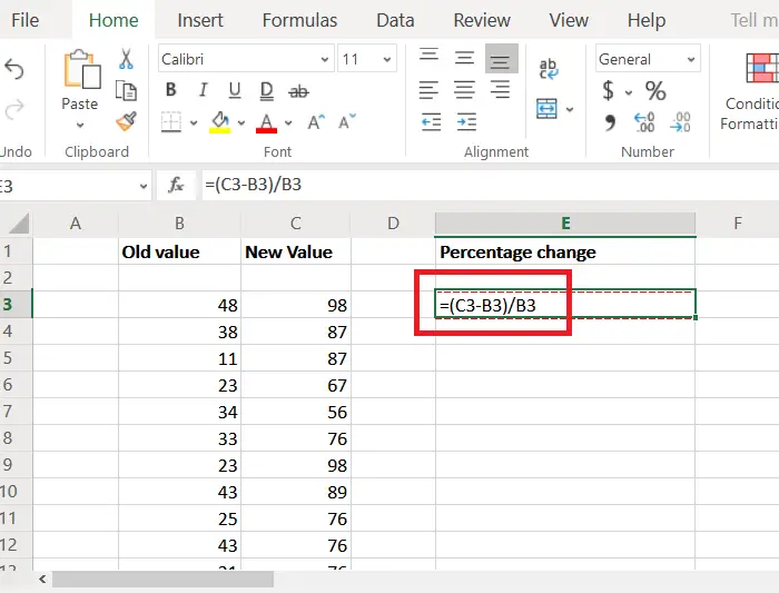
Eg. We have a range of values in columns B and C starting from row 3. Thus the first comparison values would be in cells B3 and C3.
The formula to calculate the percentage difference from cell B3 to cell C3 would become:
=(C3-B3)/B3

Where, B3 is the first cell in the range of cells across column B from which we start calculating the percentage change.
C3 is the first cell in the range of cells across column C till which we calculate the percentage change.
Let us say we need the range of cells with the percentage difference in column E. Then place the formula for finding the percentage difference in this example in cell E3.
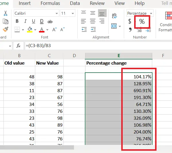
However, this would give the value in integer or decimal format. To attain the value in percentage format, please click on the Percentage button in the Number section of the Ribbon.

Again, the results are for one cell only. To pull the results down across the column, use the Fill function. Let us suppose the results are to be counted till row 16 and simultaneously till cell E16, then you would have to click on cell C3 once again.
Once it is selected, click on the small dot at the bottom right corner of the cell to highlight the Fill option. Now, without releasing the mouse click, pull the selection down to E16.
I hope it helps!
Read: Calculate Standard Deviation and Standard Error of the Mean in Excel.
Leave a Reply