Sometimes we have spreadsheets overrun with data and it can be quite cumbersome where Microsoft Excel is concerned. Not everyone wants to see the data all at the same time, so the best option to take here is to hide the columns, then unhide them whenever the data is needed.

Now, we must say that hiding columns in Excel is easier than one might have originally expected. It requires just a few clicks of the mouse button to accomplish the task.
How to hide and unhide columns in Excel
The solutions below will help you to learn how to get the job done:
- Hide selected Columns in Microsoft Excel
- Unhide selected Columns in Microsoft Excel
1] Hide selected Columns in Microsoft Excel

When it comes down to hiding columns in Microsoft Excel, this is an easy task to get done. So, without any other delays, let us explain how to do it.
- Open Microsoft Excel
- From there, launch into a spreadsheet with all the relevant data.
- If you want to select a single column, then you much click on the column header.
- For those who want to select more than one adjacent column, then drag through them. Alternatively, you can select the first column header, and from there, hold Shift, then click on the last column header located in the range.
- Finally, if you want to choose multiple non-adjacent columns, then select the first column header, and waste no time by holding Ctrl. Finish off by clicking on the leftover column headers.
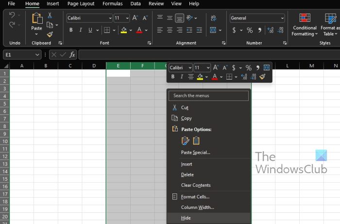
- Finally, right-click on the selected columns, then choose Hide from the context menu, and that’s it.
Bear in mind that once a column is hidden in Excel, a thick white line will appear between the remaining columns. For the many Mac users out there, this white line may appear as the color green.
2] Unhide selected Columns in Microsoft Excel
After hiding the columns in Excel, there may come a time when you will want to view them again. Therefore, it is good to learn how to unhide them for such days.
- Select the columns located on each side of the hidden columns.
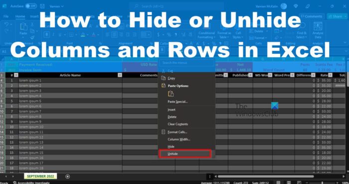
- Right-click and select Unhide from the context menu.
Alternatively, you can double-click the line that indicates the hidden columns for them to return.
How to hide and unhide Rows in Excel
Learn how to hide and unhide rows via the following steps:
- Hide rows in Excel
- Unhide rows in Excel
1] Hide rows in Excel

When it comes down to hiding rows, the steps are similar to that of hiding columns. Let us look at how to accomplish this right now.
- Highlight the rows you want to have hidden.
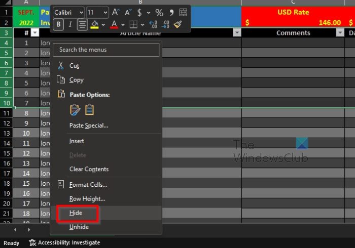
- Right-click on the highlighted rows.
- From the context menu, then, you must now click on Hide.
The rows should now be hidden from sight. But worry not because we can retrieve them.
2] Unhide rows in Excel
Returning hidden rows to visibility is an easy task that only takes a few seconds to get done.
- Highlight the rows below and above the section where the hidden rows are located.
- After that, right-click within the highlighted section.
- From the context menu, please select Unhide.
All hidden rows should now be visible again and ready for use.
READ: How to hide Row and Column Headers in Microsoft Excel
What is the shortcut key to hide and unhide columns in Excel?
You might not have known this, but there is a shortcut key for hiding and unhiding columns in Microsoft Excel. The keys in question are Ctrl + Shift + 0. But before it can work, you must first select the column you want to hide or unhide, then press the series of keys to get the job done.
How do I unhide multiple rows and columns in Excel?
To unhide or hide multiple rows and columns in Excel, you need to follow the same method as above. That said, you need to choose the columns or rows, right-click on it and select the Hide option. Alternatively, you can choose the same rows or columns, right-click on it and select the Unhide option.
Leave a Reply