How to highlight Cell or Row with Checkbox in Excel

Microsoft Excel is an application used by many around the world, especially for data analysis, due to the mathematical and statistical features it offers. In this tutorial, we will explain how to highlight a cell or row with a check box in Excel.

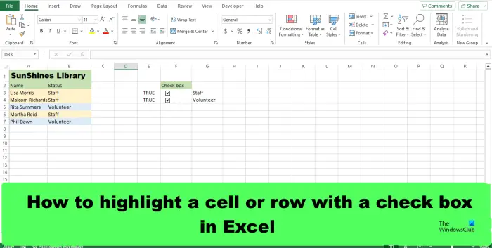
How to highlight Cell or Row with Checkbox in Excel

To highlight a cell or row in Excel, we will be using Conditional Formatting. The Conditional Formatting feature easily spots, trends and patterns in your data using bars, colors, and Icons to visually highlight important values. Follow the steps below on how to highlight a cell or row with a check box in Excel:

1. Launch Excel, then enter data.
2. Select a cell.
3. On the Developer tab, click the Insert button in the Controls group, then click the check box from the Form Controls group in the menu.
4. Draw the check box into the selected cell.
5. Right-click and select Edit Text from the menu to remove text from the check box.
6. Right-click the check box button and select Format Control
7. In the cell link box, type the cell where you want to link to the check box.
8. Highlight the cell where you want to add the conditional formatting to when the check box is selected.
9. In the Select a rule type list, select ‘Use a formula to determine which cells to format.’
10. In the ‘Format value where this formula is true’ box, type the cell where you have linked the checkbox to and add TRUE, for example: = IF ($E3=TRUE,TRUE,FALSE)
11. Click the Format button, select the Fill tab, and choose a color and then click OK
12. Click both check boxes to see the selected rows highlighted.

Launch Excel.

Enter your data.

Now we are going to insert the check boxes.

Select a cell.

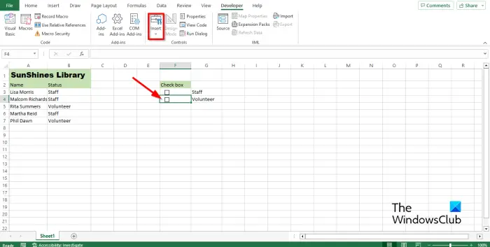
On the Developer tab, click the Insert button in the Controls group, then click the Check Box from the Form Controls group in the menu.

Now draw the check box into the selected cell.

If you want to remove the text from the check box, right-click and select Edit Text from the menu.

Now delete the text.

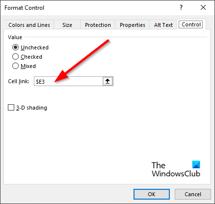
Right-click the check box button and select Format Control from the menu.

A Format Control dialog box will open.

In the cell link box, type the cell where you want to link to the check box, for example, $E3, then click OK.

Now we are going to add the conditional formatting to the cell.

Highlight the cell where you want to add the conditional formatting when the check box is selected, for instance, in the photo, we have highlighted a row containing Staff.

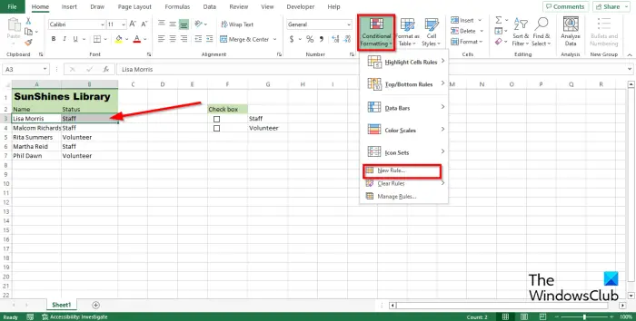
On the Home tab, click the Conditional Formatting button in the Styles group, then select New Rule from the menu.

A New Formatting Rule dialog box will open.

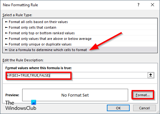
In the Select a rule type list, select ‘Use a formula to determine which cells to format.’

In the ‘Format value where this formula is true’ box, type the cell where you have linked the check box, and add TRUE, for example, = IF ($E3=TRUE,TRUE,FALSE).

Now we want to select a color.

Click the Format button, select the Fill tab, and choose a color.

Then click OK for both dialog boxes.

Follow the same method for the other cells that you want to highlight, with that color, for instance, in the photo above, highlight all the rows containing Staff.

In this tutorial, we want the rows containing ‘Volunteer’ to have a different color.

Right-click the check box button adjacent to the cell containing ‘Volunteer’ and select Format Control from the menu.

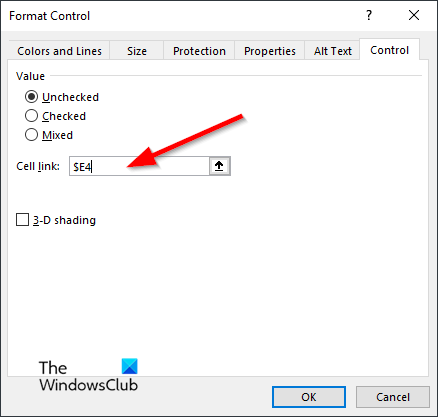
In the cell link box, type the cell where you want to link to the check box, for example, $E4, then click OK.

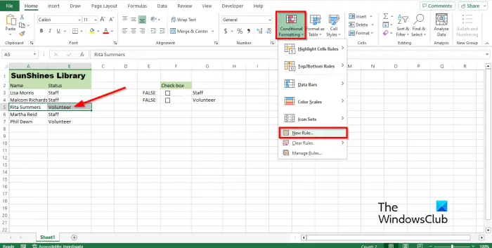
Highlight the row where you want to add the conditional formatting when the check box is selected, for instance, in the photo, we have highlighted a row containing ‘Volunteer.’

On the Home tab, click the Conditional Formatting button in the Styles group, then select New Rule from the menu.

A New Formatting Rule dialog box will open.

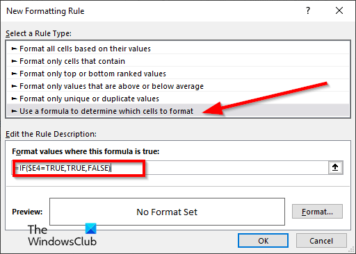
In the Select a rule type list, select ‘Use a formula to determine which cells to format.’

In the ‘Format value where this formula is true’ box, type the cell where you have linked the checkbox and add TRUE,  for example, = IF ($E4=TRUE,TRUE,FALSE).

Now we want to select a color.

Click the Format button, select the Fill tab, and choose a color.

Do the same steps for the rows you want to highlight.

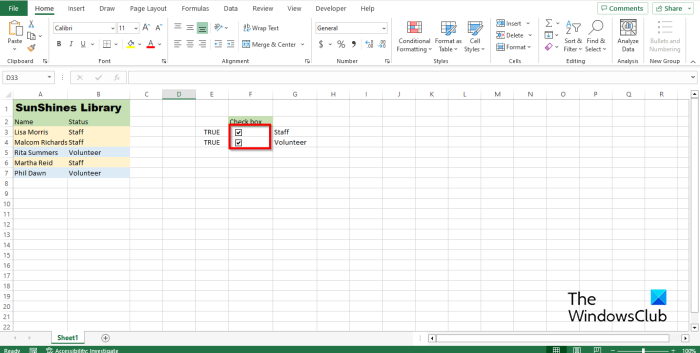
In this tutorial, you will notice that when the check box for Staff is selected, the row containing ‘Staff’ is highlighted in pink, and when the check box for ‘Volunteer’ is checked, the color of the row containing ‘Volunteer’ will turn blue.

How do I change the appearance of a checkbox in Excel?

1. Right-click the check box and select Format Control from the menu.
2. A Format Control dialog box will open.
3. Click the Colors and Lines tab. Then choose a color under the Fill section.
4. You can also change the lines and the style of the check box.
5. Then click OK.
6. The appearance of the check box will change.

READ: How to add Border in Excel

How do I add a checkbox in Excel without the Developer tab?

1. Click the Insert tab, click the Symbol button drop-down, and select Symbol.
2. In the dialog box, select the font Winding, search for the check box symbol, then click OK.
3. The symbol check box cannot be formatted like the Developer check box; it is just a symbol.

READ: How to add Alt Text in Excel

We hope you understand how to highlight a cell or row with a check box in Excel.