In this post, we will show you how to Insert a diagonal line to a cell in Microsoft Excel and Google Sheets. Diagonal lines are often used to split a cell to differentiate the headings for the first column and the top row while working with tables in spreadsheet software. They are also used to display more than one value in a cell or create multi-valued cells for audit reports. While Microsoft Excel offers a built-in way to insert a diagonal line to a cell, there’s no direct way offered by Google Sheets. Though, there are workarounds.

How to put a Diagonal Line through a Cell in Excel or Google Sheets
There could be many use cases of having a diagonal line to split data in a cell; nevertheless, learning different ways of doing this can prove to be useful if you’re a regular user of Microsoft Excel or Google Sheets.
Microsoft Excel makes it easier than ever, as it provides a feature using which you can quickly add a diagonal line to a cell. Unfortunately, no such feature is available in Google Sheets as of now. But you can still do this using some techniques we are going to explain in this article.
Split a cell diagonally in Microsoft Excel
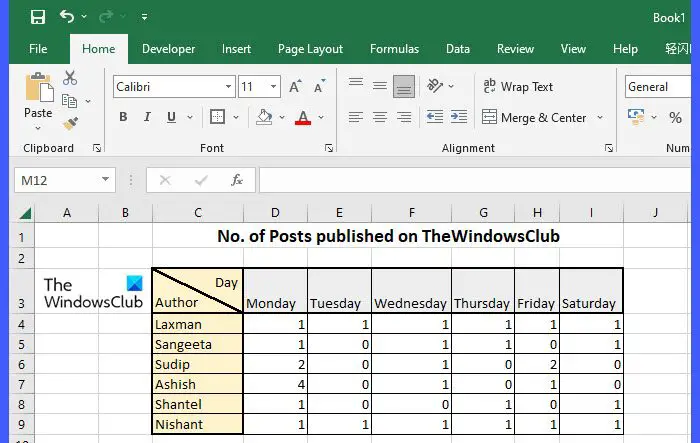
As stated above, there’s a built-in option to diagonally split a cell in Excel. However, you can also use ‘Shapes’ to insert a diagonal line into a cell. So there are 2 ways of doing this in Excel:
- Using the Border feature
- Using Shapes
Let us see these in detail.
A] Using the Border feature
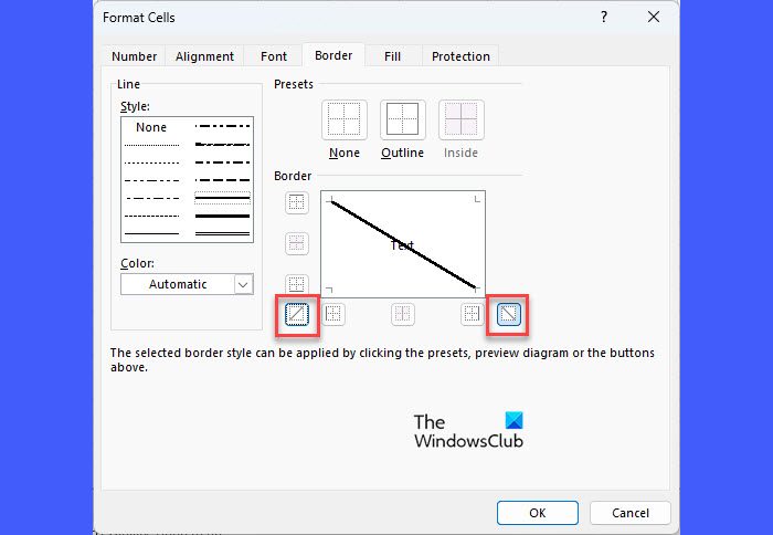
Select the cell that you want to split diagonally. Then right-click on it and select the Format Cells… option from the context menu.
In the Format Cells dialogue window, click on the Border tab. Under the Border section, you will notice two presets to add diagonal lines to the cell (top to bottom and bottom to top), as shown in the above screenshot. Select a preset to preview it. Then click on the OK button.
The diagonal line will be added to the cell. Now enter the 2 headers giving some space in between, and wrap text within the cell. After this, use the space bar or backspace to adjust the positions of both headers in accordance with the diagonal line. You may also press Alt+Enter, keeping the mouse cursor before the second header to stack it below the first header.
To remove the diagonal line, select None under Presets in the Format Cells window.
B] Using Shapes
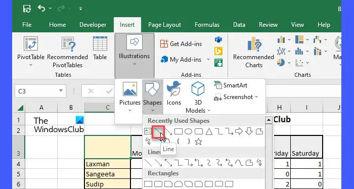
Click on the Insert tab at the top of the spreadsheet. Then click on Illustrations > Shapes, and select the Line tool. Your mouse cursor will change into a plus (+) icon. Take it to the cell which needs to be split diagonally. Make a left mouse click, hold it, drag it to draw a line, and then release the click when the line is drawn. Change the color of the line using the Shape Format options.
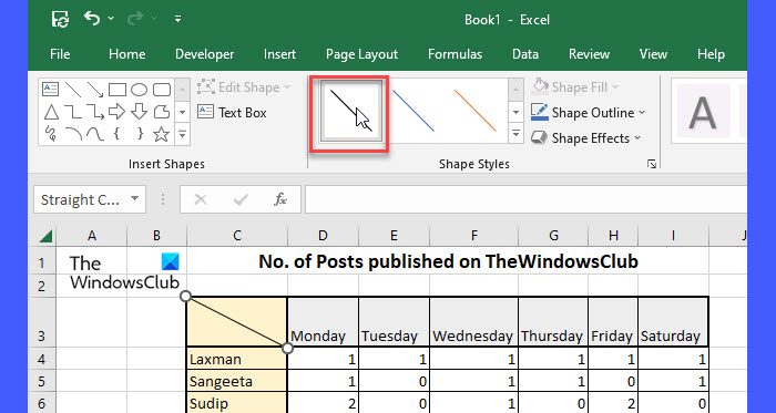
Now add the headers as described above.
This is how you insert a diagonal line to a cell in Microsoft Excel. Now let’s see how to do this in Google Sheets.
How to Insert a diagonal line to a cell in Google Sheets
Split a cell diagonally in Google Sheets
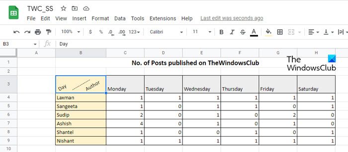
In Google Sheets, you can use the following features to insert a diagonal line to a cell:
- Using the Text Rotation feature
- Using the Drawing feature
- Using the SPARKLINE function
Let us see these in detail.
A] Using the Text Rotation feature
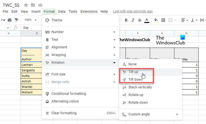
Text Rotation is a feature of Google Sheets that allows rotating the content of a cell. It not just tilts the text, but also offers a custom angle option to define the degree of rotation. You can use this feature to add a diagonal line to a cell.
Select the cell where you’d like to insert a diagonal line. Then enter the first header. Press the Alt key, hold it, and press Enter. The cursor will come to the beginning of the next line within the same cell. Draw a line using dashes (——-). Again press Alt+Enter to bring the cursor to the next line and then type the second header.
Now Click on the Format menu on top and select Rotation > Tilt up/ Tilt down.
This will rotate the line diagonally, along with the text. By default, the content of the cell will be rotated at 45 degrees. You can change this and apply a different angle of rotation to the cell using the Custom angle option.
Please note that if the cell has borders, they will also be rotated along with the cell content and make the whole arrangement look displaced. In that case, you may use the next method to diagonally split a cell in Google Sheets.
B] Using the Drawing feature
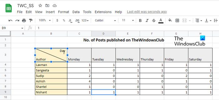
The Drawing tool allows you to create a drawing or an illustration on a blank canvas using shapes, images, etc., and insert it into your spreadsheet.
Select the cell which needs to be split diagonally. Enter the 2 headers using Alt+Enter as described above, and use the space bar to adjust their position within the cell.
Now click on the Insert menu on top and select the Drawing option.
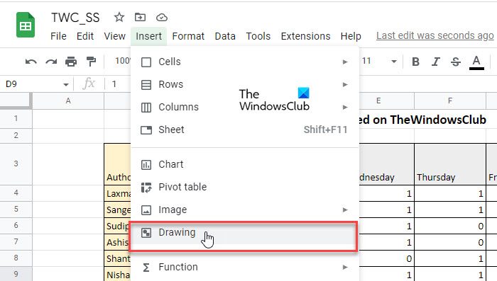
You will be presented with a blank canvas. Select the Line tool from the toolbar on top of the canvas. Using your mouse, draw a diagonal line on the canvas. Then click on the Save and Close button.

The line will appear on top of the selected cell. Click on the line to select and resize it. Resize the line to fit the cell. This way, you can insert more than 1 diagonal line into a cell in Google Sheets.
Read: How to insert WordArt in Google Sheets using Google Drawings.
C] Using the SPARKLINE function
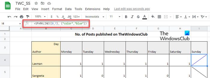
The Sparkline function is used to create miniature charts that can fit within single cells. It represents a trend based on the numerical data of a selected range of cells. This trend can take up 3 different forms: line, column, and bar. We can use the ‘line’ form to create a diagonal line within a cell in Google Sheets.
SPARKLINE function has the following syntax:
= SPARKLINE(data, [options])
Where data refers to the cell range containing the numeric data, and options are additional settings used to customize the sparkline chart.
Before we proceed, please note that the SPARKLINE function takes up the entire cell, so you can’t enter any value in the cell. So this method will basically insert a diagonal line in a blank cell in Google Spreadsheets.
Click on the desired cell and type the following function to draw a diagonal line from top to bottom:
=SPARKLINE({1,0})
Press the Enter key. The cell will split diagonally. In the above function, we have passed 2 datapoints as 1 and 0. So the function will create a diagonal line as a result.
To draw a diagonal line from bottom to top, type the following function in the cell:
=SPARKLINE({0,1})
You can change the color of the line using the color argument as follows:
=SPARKLINE({0,1}, {"color","blue"})
You can also adjust the height and width of the cell to adjust the size of the line.
Hope you find this post useful. Do let us know in the comments section below if you have any issues.
Read Next: How to add a Tooltip in Excel and Google Sheets.
Leave a Reply