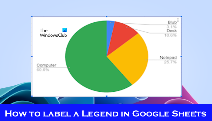
In this article, we will show you how to label a Legend in Google Sheets. Labels focus on individual things, providing names or identifiers. Legends explain systems or groups of things, providing contextual information.

How to label a Legend in Google Sheets
Sometimes when you work with charts and you want to make your charts easier to understand. You can do so by adding proper label legends. We will show you how to label a legend in Google Sheets, using the following methods described below:
- Create a chart
- Edit the text of Legend Label
Let’s start.
1] Create a chart
To label a legend, first, we have to create a chart:

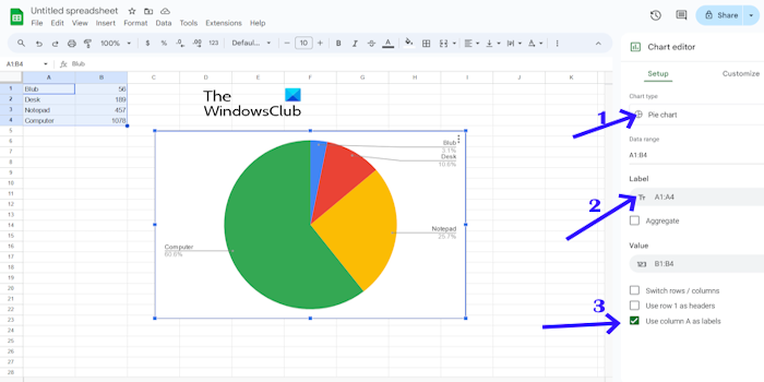
- First, enter your graph’s data into a column or row in Google Sheets.
- Highlight the data by holding the left mouse button and dragging the cursor over the data entered to select it.
- Click on the Insert tab and select Chart to add the graph to the sheet. Google Sheets selects the chart type by default. You can change it by clicking the Chart type drop-down menu to select one of the Pie graph types that you want to add a label legend to.
- Click in the Add Label box, and select the cell range that includes your chart data. Then the chart will display the data value labels as shown in the above image.
- If you want to remove the label legend by deselecting the Use column A as labels checkbox.
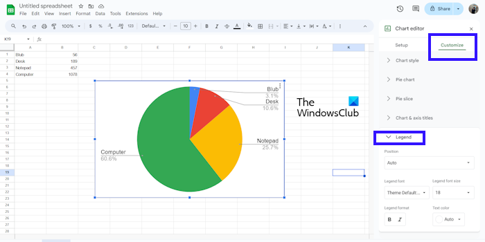
You can also adjust or modify the Location of the Legend in your Chart. To do so use the below steps:

- Click on Customize next to the Setup tab.
- Click on Legend.
- Select the position as per your choice.
- You can change the text color, legend size, legend font, and legend format.
2] Edit the text of Legend Label
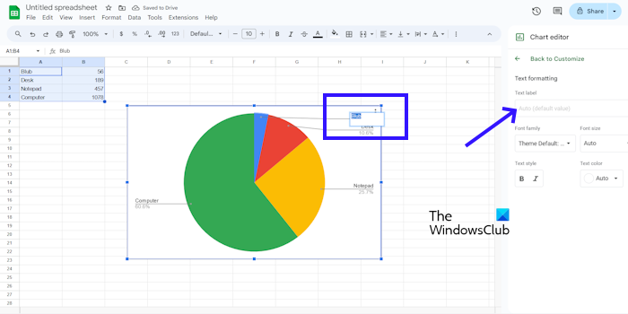
If you want to make your chart more representable, then you can edit the text of each legend label. Use the following steps to edit the text of the Legend Label:

- Double-click on the label you want to edit within the chart.
- This will open the ‘Text Formatting’ options for the label in the Chart editor.
- Now, enter the new text you want to use. You can also change the formatting for that specific label by choosing your desired font family, size, style, and color.
That’s it and I hope this helps.
How do I rename a legend in Google Sheets?
If you want to rename the entire legend in Google Sheets, double-click the chart to open the Chart editor. Now, click on the Customize tab on the right panel. Open the ‘Text Formatting’ options for the label in the Chart editor. After that, enter the new text you want to use. If you want to edit individual data series in the legend, double-click the chart to open the Chart editor, then double-click on the specific data series legend entry you want to rename. A small text box will appear. Now, enter the new text you want to use.
How do I add a title to my legend?
To add a title to your legend, click on the Insert tab. Select Chart and click on Customize. Now, select the Chart & axis title. You can add your title in the Title text.
Read next: Create Animated Graphs and Charts online free.
Leave a Reply