How to make an Attendance Sheet in Excel

In this article, I will show you how to make an attendance sheet in Microsoft Excel. This tutorial will help you manage the attendance records digitally. By using this automated Excel sheet, you can easily calculate the percentage of present days of your employees, which will help you when your employees’ appraisal is due.

How to make an Attendance Sheet in Excel

This guide will help you create an attendance sheet in Excel. It is beneficial for both schools and organizations.

I have created a sample sheet containing the names of some employees. If you create an attendance sheet for your school, you can replace the Employees’ Names field with the Students’ Names field. You can also use the Wrap Text and Merge & Center options to arrange text properly in the cells.

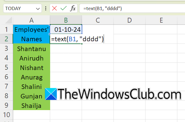
The first step is to add the dates of a particular month to the Excel sheet. Select a cell and type the date with the format DD-MM-YYYY. For example, to create the attendance sheet for October 2024 month, the date will be 01/10/2024. The cell below the date should represent the respective day. For this, type the following formula in the cell just below the cell containing the date:

=TEXT(B1, "dddd")

In the above formula, B1 is the cell’s address containing the date. Your Excel sheet may have a different address.

The next step is to format the date only in the DD format. This will make your attendance sheet look compact. Right-click on the cell containing the date and select Format Cells. Select Custom and select the dd-mm-yy format on the right side. Delete the mm-yy from that format and click OK. If you want to represent the days’ names in short format, change the above formula to:

=TEXT (B1, "ddd")

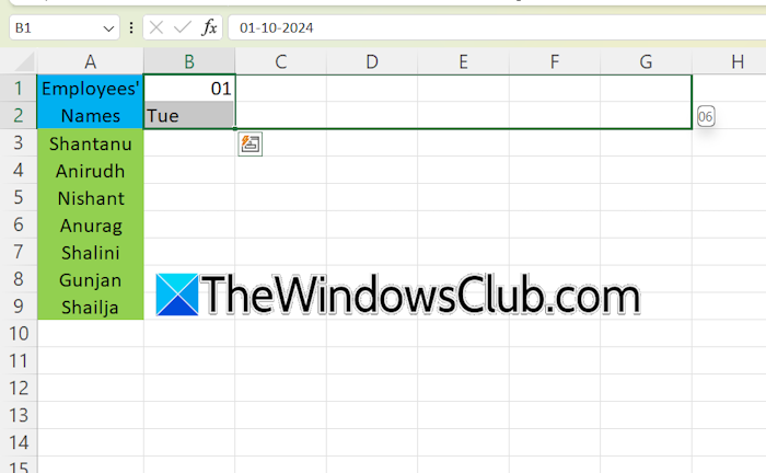
Select the cells containing the date and day and drag them to the right using the Fill Handle. After filling up all the dates of a month, enter the following texts in the next cells:

Present
Absent
Holidays
Working Days
Attendance in Percentage

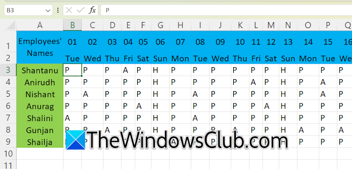
Represent Sundays with the letter H, present days of your employees with the letter P, and absent days of your employees with the letter A.

The next step is to apply the Conditional Formatting for the present days, absent days, and holidays. I have selected green to show the present days, yellow for the absent days, and red for holidays. You can select the color accordingly.

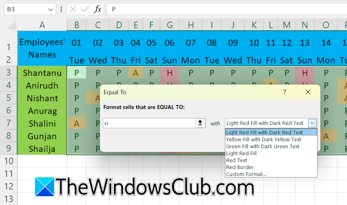
Select all the cells containing the letters P, A, and H. Go to Home > Conditional Formatting > Highlight Cells Rules > Equal To. Type P in the required field and select the required option in the drop-down. Repeat this process to apply the Conditional Formatting for the cells showing holidays and absent days. You can also select a custom color for the cells by selecting the Custom Format option.

To calculate the Present days of an employee, select the required cell and enter the following formula:

=COUNTIF(cell range, "P")

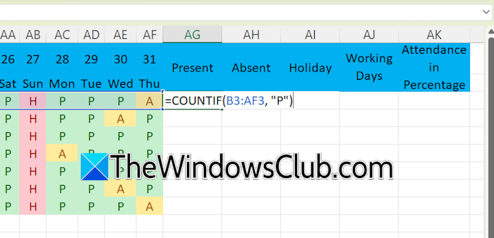
In the above formula, type the correct cell range representing all the total days of a month for each employee. For example, if an employee’s total days of a month ranges from B3 to AF3, the cell range will be B3:AF3. Hence, the formula will become:

=COUNTIF(B3:AF3, "P")

Fill the data in all empty cells using the Fill Handle. Similarly, count the absent days of an employee by using the following formula:

=COUNTIF(cell range, "A")

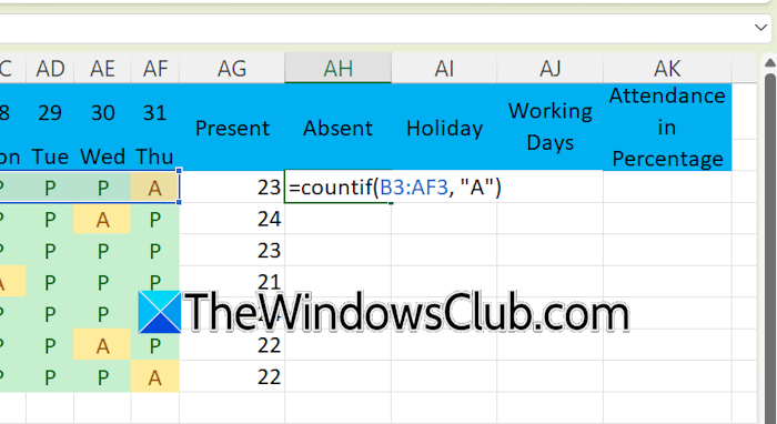
Enter the correct cell range in the above formula; otherwise, you will get an error or incorrect result.

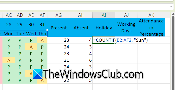
In this Excel sheet, holidays are the total count of Sundays in a particular month. Therefore, select the cell range containing the days’ names to count holidays. Use the following formula:

=COUNTIF(cell range, "Sun")

Type the correct cell range. In the above formula, you must also fix the cell range; otherwise, Excel will change the cell range values when you fill other empty cells using the Fill Handle. In this case, use the $ function.

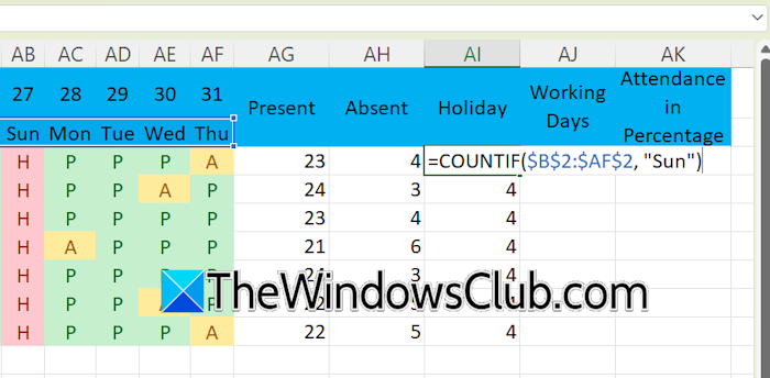
Suppose the cell range containing the days’ names is from B2 to AF2, the formula will be:

=COUNTIF($B$2:$AF$2, "Sun")

Working days are the total of present and absent days. Therefore, the formula to calculate the working days is:

=SUM(cell range)

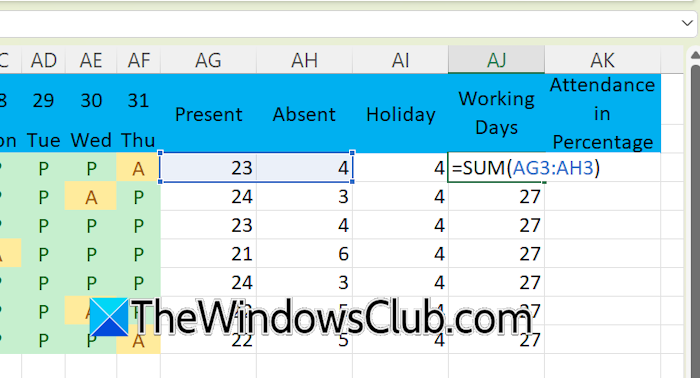
Let’s say, the present and absent days of a particular employee are displayed in the cells AG3 and AH3 respectively, the formula will become:

=SUM(AG3:AH3)

To calculate the attendance percentage of an employee, use the following formula:

=Present days/Working days

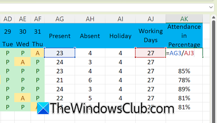
Replace the present days and working days in the above formula with the correct cell address. You will get the result in decimals. Convert it into percent value by % style under the Home tab. Alternatively, you can use the Ctrl + Shift + % keyboard shortcut. Use the Fill Handle to fill the empty cells.

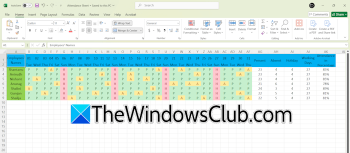
The attendance sheet in Excel for a particular month has been created. To create the attendance sheet for the next month, copy the entire data to a new page in Excel and change the dates. The respective days’ names will change automatically. Now, you have to enter P, A, and H manually.

That’s it. I hope this helps.

How do I create a checklist box in Excel?

The Checklist feature is available in Microsoft Office 365 and Excel for the Web. To create a checklist box in Excel, go to the Insert tab and click on the Checkbox option. The checkbox will then be added to the selected cell or cell range.

In Office versions other than Office 365, two different types of checkboxes are available: ActiveX Control checkboxes and Form Control checkboxes. These checkboxes are different from those available in Microsoft Office 365.

How to print an Excel sheet?

To print an Excel sheet, open that sheet in Excel, then go to File > Print. Alternatively, you can also use the Ctrl + P keyboard shortcut. Select your printer, adjust the print settings, and click Print.