Is it frustrating that the leading zeros are automatically removed from your Excel workbook? Excel typically removes the leading zeros before a number as you input the number in a cell. It treats cell entries lacking explicit formatting as numeric values by default. And leading zeros are often deemed insignificant in numeric formatting and are consequently omitted. Also, leading zeros can cause problems in some numeric operations. So, the zeros are automatically deleted.
If you want to keep the leading zeros in Excel as it is to input numeric data like account numbers, postal codes, phone numbers, etc., this post will show you how.

How do you allow zeros in front of numbers in Excel?
There are different methods to keep the leading zeros in a number in an Excel workbook. To do that, you can set the format of the cells accordingly or use the TEXT function for the target cells. Besides that, you can even write a VBA script to stop Excel from automatically formatting cell values and deleting the leading zeros.
How to prevent Excel from removing leading zeros
If you want to prevent Excel from removing leading zeros in your workbook, use the below methods:
- Add an apostrophe before the number.
- Format cells as text.
- Set a Custom format.
- Use Special formats.
- Use the Get & Transform feature.
- Apply the TEXT function.
1] Add an apostrophe before the number
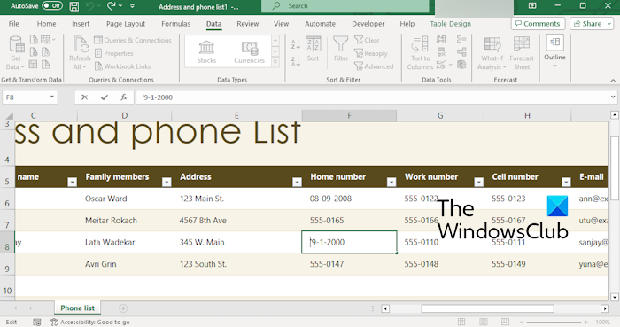
One of the easiest methods to stop Excel from deleting leading zeros is to insert an apostrophe before the actual number. The number will be displayed without the apostrophe symbol.
While this straightforward method is good for small datasets, manually entering apostrophes can become tedious and error-prone, especially when dealing with large amounts of text or data entry tasks. In that case, we have some other methods that you can use.
Read: How to get real-time Currency Exchange Rates in Excel?
2] Format cells as text
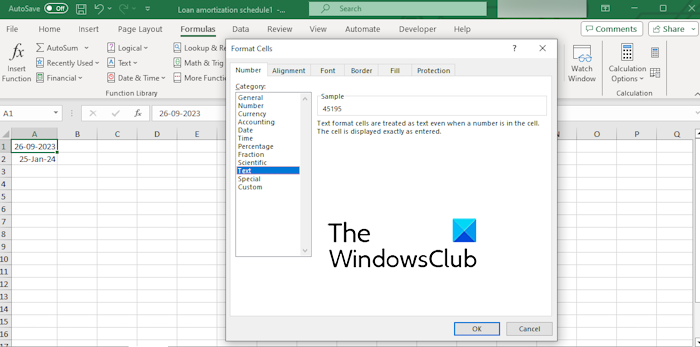
The next method you can use to prevent the removal of leading zeros in Excel is to format the target cells as Text. When done that way, the number will be displayed as you type and won’t be automatically formatted.
- First, select the target cells or an entire column in your workbook and then right-click on them.
- Next, click on the Format Cells option from the context menu. To open the Format Cells dialog, you can also use the CTRL+1 shortcut key.
- After that, under the Numbers tab, select the Text category from the Numbers tab.
- Finally, click on the OK button to save changes.
See: How to remove Scientific Notation in Excel?
3] Set a Custom format
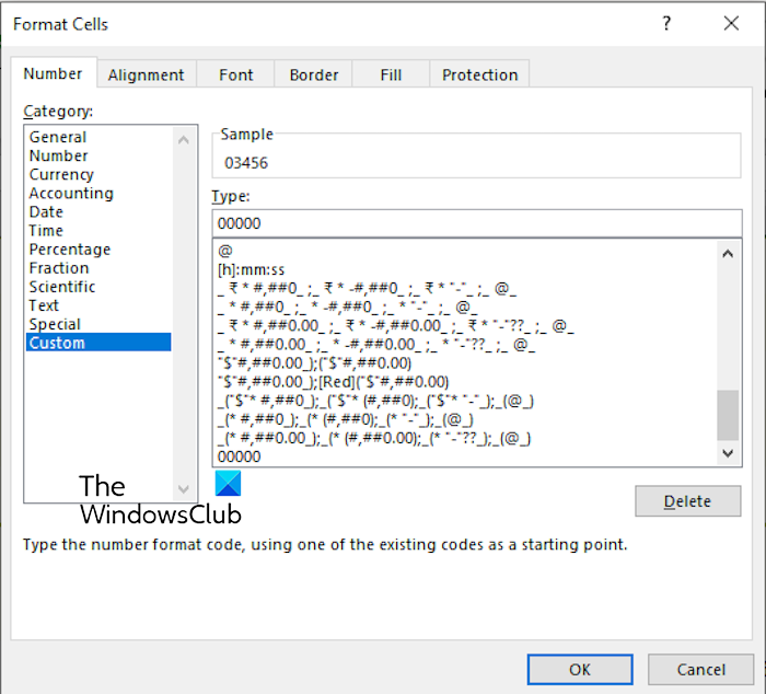
You can also use a Custom format to enter number codes like Social
security, postal code, etc., that contain less than 16 digits in Excel.
- First, select the problematic cells and press CTRL+1 to open the Format Cells prompt.
- Under the Number tab, click on the Custom category.
- In the Type box, type the number format e.g., 000-00-0000, 00000, etc.
- Once done, press the OK button to save the new format.
Read: How to lock cells in Excel formula?
4] Use Special formats
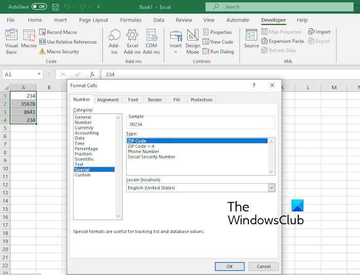
Excel has some built-in formats to input number codes, including ZIP codes, phone numbers, and social security numbers. So, to input a particular type of number, you can use the respective format. For that, select the cells and press CTRL+1. Then, select the Special category and choose the desired type from the available ones. Once done, press the OK button to save changes.
5] Use the Get & Transform feature
If you are importing datasets from external files, you can prevent Excel from deleting the leading zeros by using the Get & Transform feature. The source file can be in the format of Text, XML, Web, JSON, etc.
Here’s how to do that:
First, open your Excel workbook and go to the Data tab.
Now, click the Get Data drop-down button and choose the From File > From Text/CSV option or the file format you want to import.
Next, browse the input file and click on the Import button to import the file.
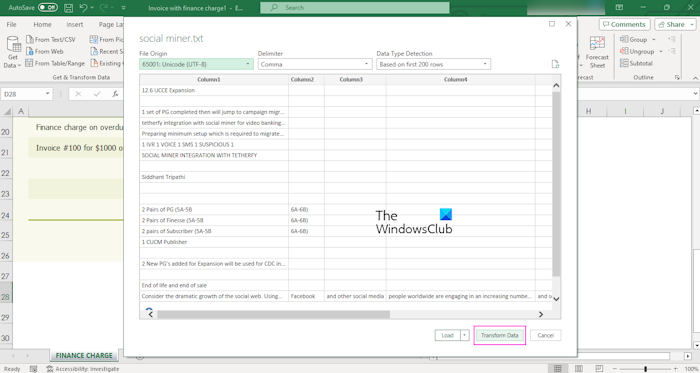
In the opened dialog, press the Transform Data button.
After that, in the Power Query Editor window. choose the columns you want to edit and go to the Transform menu.
Now, click on the Data Type button and then select Text.
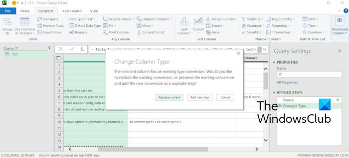
In the Change Column Type prompt, click the Replace current button and let Excel convert the selected column data format to text.
Once done, press the Close & Load button to return to Excel.
The imported dataset will now have leading zeros in them.
You can use the Data > Refresh feature to update the data automatically.
Read: How to add Camera tool in Excel?
5] Apply the TEXT function
Another method you can use to keep the leading zeros in Excel is to use the TEXT function. For example, if you want to insert a social security code in the E1 cell, you can use the “=TEXT(E1,”000-00-0000″)” function. Similarly, you can use this function from other number codes.
If you have a command over Excel functions, you can also use other functions besides the TEXT function to retain the leading zeros. Here are some examples of such functions:
- A combination of REPT and LEN functions, e.g., “=REPT(0,5-LEN(A5))&A5“
- CONCATENATE Function, e.g., “=CONCATENATE(“00”,A5)“
- RIGHT function with Ampersand operator (&), e.g., “=RIGHT(“00000″&A5,5)“
Similarly, there are other functions that can be used for the same.
Read: How to add Text to a Cell in Excel using Formula?
How do I open Excel without losing leading zeros?
If you are trying to import an existing Excel file to your workbook without removing leading zeros, go to the Data tab and click on the Get Data > From File > From Excel Workbook option. Now, choose the source file, press the Import button, and then click on Transform Data. Next, select the target columns, go to the Transform tab, and set the Data type to Text.
Now read: How to open Apple Numbers file in Excel?
Leave a Reply