In this post, we will show you how to remove the green triangle in Excel. A green triangle is a small marker that appears in the upper-left corner of a cell, signaling a potential issue with the cell’s contents. It is part of Excel’s Error Checking feature and is designed to help users identify and address potential issues or inconsistencies in their data.
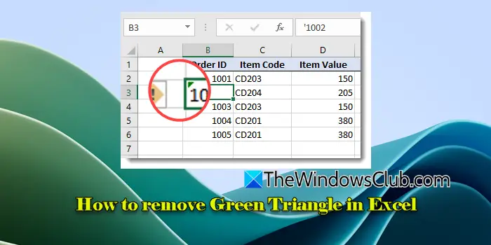
While the green triangle helps ensure data accuracy, some users may find it unnecessary, especially when they are confident about their work. In such cases, they might prefer to remove or disable the green triangles and ignore the errors.
How to remove Green Triangle in Excel
If you’d like to remove the green triangle in Excel, you should know common reasons why the triangle appears.
The most typical triggers for the green triangle are:
-
Formulas inconsistent with other formulas: This occurs when a formula differs from those in adjacent cells, potentially causing calculation issues.
-
Numbers formatted as Text: When numbers are entered as text, Excel flags them because it can interfere with calculations.
-
Formula error: Excel detects a possible error in a formula, such as the Divide by Zero error or incorrect cell references.
Knowing what triggers these warnings, you can take appropriate action to switch off background error checking, correct mistakes, or confidently ignore the indicators when they are unnecessary.
1] Switch off background error checking
To turn off the green triangles altogether, follow these steps:
Go to the File menu and select Options. In the Excel Options window, click on Formulas in the left pane. Under Error Checking, you’ll see a checkbox for ‘Enable background error checking‘. Uncheck this box and click OK to save changes.
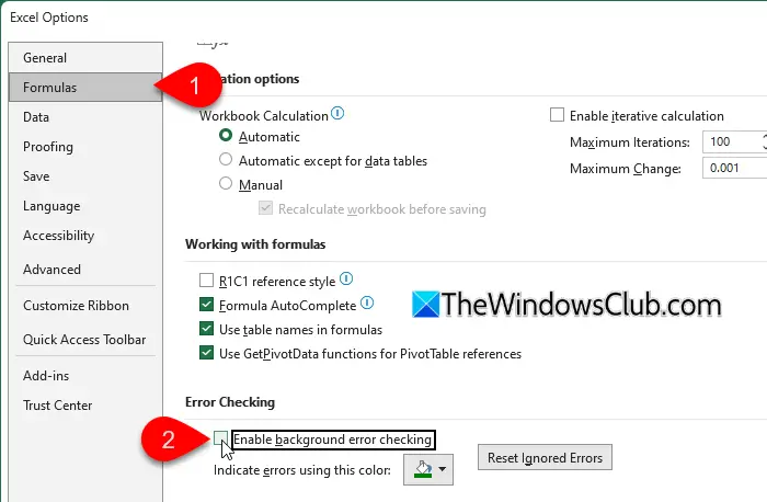
Excel will no longer automatically scan for and flag potential errors in the current workbook you’re working on, as well as in any other workbooks you open in the future.
You also have the option to selectively turn off specific error-checking rules that Excel applies by default, rather than disabling the entire background error checking feature. This way, you can eliminate specific alerts that may be unnecessary to you while still retaining the ability to receive notifications about other potential errors.
To selectively turn off specific error-checking rules in Excel, uncheck the specific rules you want to disable under the Error Checking section.
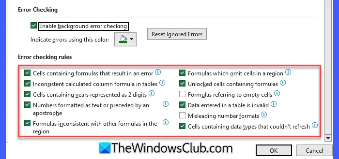
For example, you can uncheck:
- Numbers formatted as text or preceded by an apostrophe
- Formulas which omit cells in a region
- Other options as needed
Once you’ve made the changes, click OK and close the Excel Options dialog box. This will remove green triangles from the cells that are flagged by the specific error-checking rules you have disabled.
2] Fix the error
If the error indicates a logical mistake, such as a Divide by Zero error, it’s crucial to resolve it to avoid misleading outcomes.
To fix the error, you can use the Trace Error button (a small warning icon that appears next to the selected cell). When you click the Trace Error button, a drop-down menu appears with a tailored set of options depending on the nature of the error. You can choose the desired option to resolve the specific issue indicated by the error.
For example, if it is a Divide by Zero error (denoted as #DIV/0!), you can choose Show Calculation Steps. This option allows you to see how Excel arrived at the error, helping you understand the context and identify what went wrong in your formula. Or you can choose Edit in Formula Bar. By clicking this option, Excel places the formula into editing mode in the formula bar, allowing you to make direct adjustments.
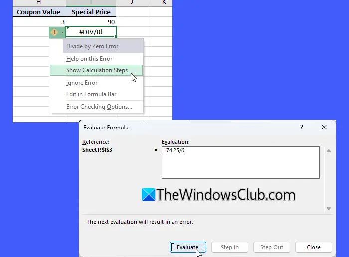
Similarly, if it is a Number Stored as Text error, you can choose Convert to Number to change the text-formatted number into a proper numeric value or choose Edit in Formula Bar to manually remove any leading apostrophes or make necessary adjustments to the value.

3] Ignore error
When you are certain that the data is accurate and the error indicator is irrelevant to your analysis, you may ignore the error. However, ignoring an error is more of a temporary solution. If the contents of the cell change in the future, Excel might flag it again if the same error condition arises.
To ignore an error, select the cell that contains the green triangle and click the Trace Error button. Select ‘Ignore Error‘ from the menu that appears.
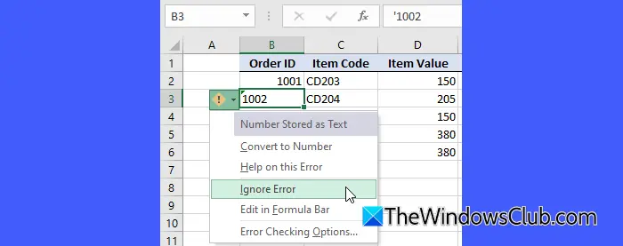
Ignore Error only applies to the selected cell or cells and does not affect the overall error-checking settings for your workbook.
I hope this helps.
Read: How to change the color of an error indicator in Excel.
What is the green triangle in Excel?
A green triangle in Excel is a warning symbol that appears in the upper-left corner of a cell to signal an error or inconsistency in the data entered. It does not indicate that the data is incorrect or that it will cause issues; it simply serves as a prompt for you to review the cell and decide whether any action is needed.
Why do some Excel cells have a green triangle?
If your Excel workbook contains cells having green triangles, there might be potential errors or inconsistencies in the data or formulas within those cells. Select a cell and hover over the warning icon to see a hint that explains the specific issue. Additionally, by clicking on the icon, you can open a drop-down menu that provides possible options to address the error.
Read Next: How to fix the #NULL error in Excel.