Excel is one of Microsoft’s most popularly used productive software. There are lots of tips and tricks that will enhance your Excel use. Learning how to remove numbers in Excel from the left is a neat trick to automate subtracting unwanted digits. You can use this in cases where you want to delete area codes from phone numbers etc.
How to remove Numbers in Excel from the left
The ways to easily remove numbers from the left in Excel are not unique to numbers. You can use this same formula to remove other characters from a string of values in Excel. You can also use the Right function, where you tell Excel to delete the numbers on the left and keep the numbers on the right. You would specify the number of numbers you want to be deleted from the left. This is great for cases where you know the length of the numbers, for example, telephone numbers or ID numbers. Keep reading to see how this is done and how you can put it to practical use.
1] Open and prepare Excel
This is the first step where you will open Excel. To open Excel go to Start then type Excel, and click on the Excel Icon. This will open Excel for you to open a new document or open a recent document.
2] Enter the numbers in Excel cells
You may have an Excel file where you have the numbers that you want to work on. If you do not have an Excel file with numbers, this is where you will enter the numbers and other information that you may want.
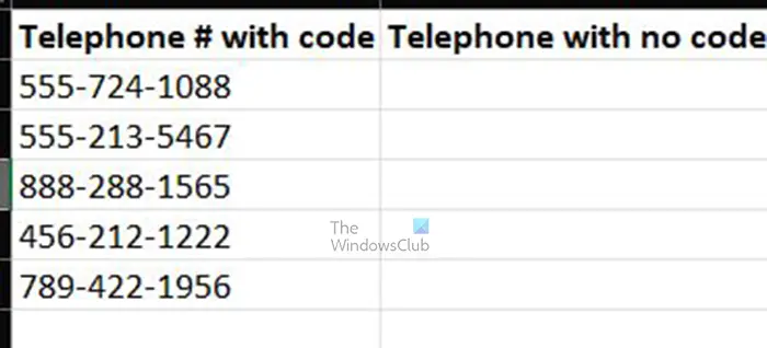
This is the Excel table with the information that will be used for the demonstration.
3] Enter the formula in the output cell
Now that you have the information in Excel, it is time to delete the left. You will place the result in an output cell. The output cell in this case is the cell under the heading Telephone with no code.
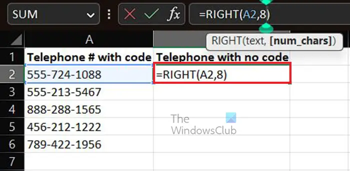
This is the formula that you will type in to delete the left numbers and output only the specified numbers to the right. The number 8 in the formula tells Excel to leave 8 characters counting from the right and delete the remainder.
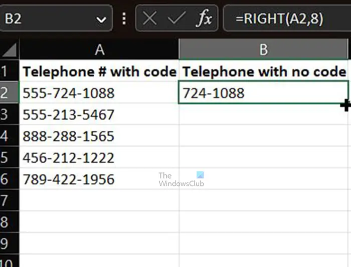
This is the result for the first row of information
4] Duplicate the results
With the first row above formulated how you want it, it is time to duplicate the formula so that the calculations will be automatic.

To easily duplicate, hover the cursor under the right lower corner of the cell. The cursor will be converted to the Plus + symbol, click, hold, and drag down to where you want to go.
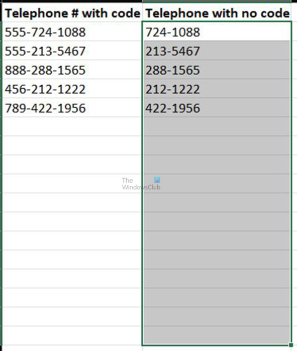
You will see the cells selected.
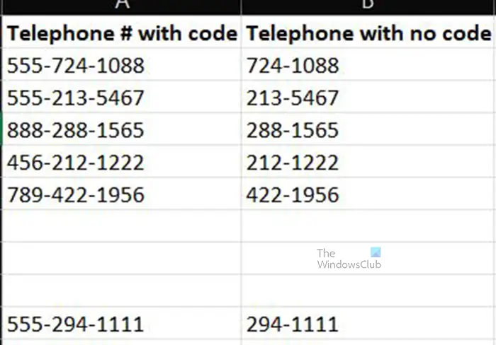
If you plan on adding additional phone numbers, drag the formula down beyond where the present numbers are. You will not see any results since the corresponding cells are blank. However, as soon as you enter numbers in the first cell, it will automatically format the numbers according to what you specified.
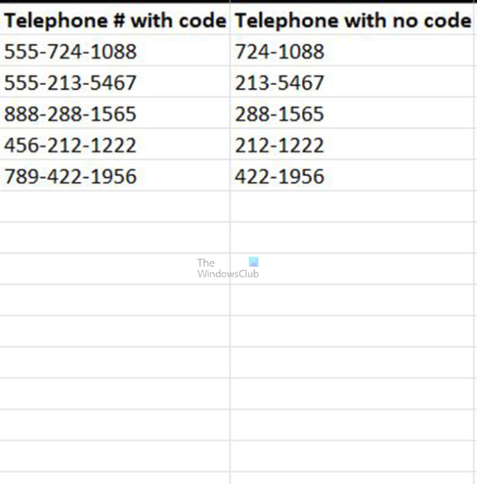
This is the completed Excel table.
Read: How to use Slicers to filter Data in Excel
What is the Trim function in Excel?
The Trim function in Excel is used to remove all spaces from text except for single spaces between words. The Trim function should be used especially on text that you have received from another application that may have irregular spacing.
What is the MID function in Excel?
The MID function is used to display the string in the middle of a line of text. The start point of the middle point would be specified by the user. Here is the formula for using MID: =MID, location of text, the starting number, the number of characters. Here is an example of how you would write the formula: =MID(B1,10,15).
Leave a Reply