In this post, we will show you how to reorder multiple columns in Power Query with Drag & Drop. Often when importing data from various sources, columns may not be in the desired order. Reordering columns not only allows you to arrange them in a logical order that aligns with your analysis or reporting needs, but also improves the readability of the data and expedites tasks such as filtering, sorting, and performing calculations.

How do you rearrange multiple columns in Excel?
You can rearrange columns in Excel by selecting the column header and dragging it to the desired position. However, if you have a large table with a lot of columns that you have to drag and scroll through, you can use the Power Query Editor. The Power Query Editor allows you to select multiple columns in the order you want to place them and then drag the columns together to their desired location.
How to reorder multiple columns in Power Query with Drag & Drop
To reorder multiple columns in Power Query with Drag & Drop, you have to follow these steps:
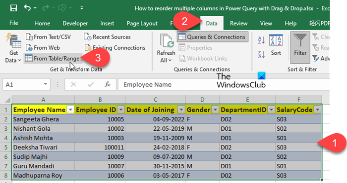
Let us say we have a sample data source as shown in the screenshot below. So the first thing we need to do is to open it in the Power Query Editor. Select the data source and click on the From Table/Range option within the Get & Transform Data section under the Data tab.

Reorder multiple columns with Drag & Drop
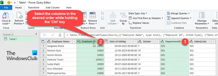
Once the data is open in the Power Query Editor, hold the Ctrl key and select the desired columns in the order you want them to be displayed. For example, to rearrange DepartmentID and EmployeeID in the following manner:
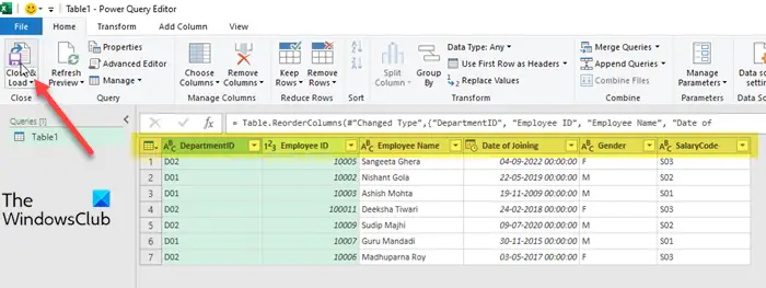
DepartmentID, EmployeeID, Employee Name, Date of Joining, Gender, Salary Code
I will select them in the order as shown in the screenshot below:

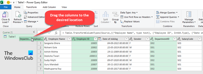
After selecting the columns, click and hold the left mouse button on any of the selected column headers, and drag the pointer to the location where you want to place the columns. Release the mouse button to drop the columns into their new position. They will be rearranged in the desired order.

Finally, click on the Close & Load button in the top menu of the Power Query Editor to apply the changes and load the reordered data back into your worksheet.

Note:
- If you want to rearrange all the columns in your data source, you must drag the selection to the right of the last column and then release the mouse button. Nothing will happen if you drag the columns to the left.
- To reverse the order of columns in your data source, select the last column, hold the Shift key, and select the first column. Then click and hold the left mouse button on the last column header and drag the pointer towards the right. Release the mouse button and the column order will be reversed. You may follow the same steps to reverse the order of just a few columns. This allows dragging the selection to the left as well.
- To ‘undo’ the reorder, right-click on the Reordered Columns step under ‘Applied Steps’ in the Query Settings panel on the right and select Delete.
An alternative method to reorder columns in Power Query
When you reorder the columns in Power Query, a Table.ReorderColumns function will be created. You can also rearrange multiple columns at once by modifying the formula text within the Table.ReorderColumns function (If you’re not able to see the function, right-click on any column header and select Move > Left/Right/To Beginning/ To End from the context menu).
Place your cursor in the formula bar on top and edit the formula text by typing the column titles in the desired order. Keep the titles within double quotes, separated by a comma. Delete the previous entries for the columns you’ve added and press Enter to apply the changes.
So this is how you can quickly reorder multiple columns in Power Query, without having to move each column individually. I hope you find this useful.
Read: Power BI Unable to connect, We encountered an error while trying to connect.
How do you sort columns in Power Query?
Open the data source in Power Query Editor and select the column you want to sort. Then go to the Home tab and click on the ‘Sort Ascending’ or ‘Sort Descending’ option within the Sort section. Alternatively, click on the dropdown next to the column header and select Sort Ascending/Sort Descending from the popup that appears. You can also use this popup to further customize the sorting by specific values or to clear the sort.
Read Next: How to switch Rows and Columns in an Excel Chart.