In this post, we will show you how to round numbers in Google Sheets. Spreadsheet data often consists of decimal numbers that lie between whole numbers. A decimal number consists of a decimal point (or a dot) that separates a whole number from its fractional part. It is often a good idea to round off numbers to a certain decimal place so that it becomes easier to work with fractional data. Rounding is used to simplify the numbers by shortening the number of digits on the right of the decimal point. It also makes the data look more uniform or symmetric. In this post, we will show you how to round numbers in Google Sheets using seven different methods.
How to Round Numbers in Google Sheets
You can round numbers in Google Sheets using the following methods:
- Round numbers using the ROUND function.
- Round numbers using the ROUNDUP function.
- Round numbers using the ROUNDDOWN function.
- Round numbers using the MROUND function.
- Round numbers using the INT function.
- Round numbers using the FLOOR function.
- Round numbers using the CEILING function.
Let us have a detailed look at each of these methods.
1] Round numbers using the ROUND function
The ROUND function rounds a number to a specific number of decimal places as per the standard rules, which are as follows:
- If the digit to the right of the rounding digit is less than 5, the rounding digit is left unchanged (rounded down).
- If the digit to the right of the rounding digit is greater than or equal to 5, the digit is increased by 1 (rounded up).
The syntax of the Round function is:
ROUND(value, [places])
- Where value refers to the number that needs to be rounded, and
- [places] refers to the number of decimal places to which the number should be rounded. It is an optional argument. If not specified by the user, it takes the value zero (0).
Now let us understand how to round numbers in Google Sheets using the ROUND function.
A] Round numbers to the right of the decimal point
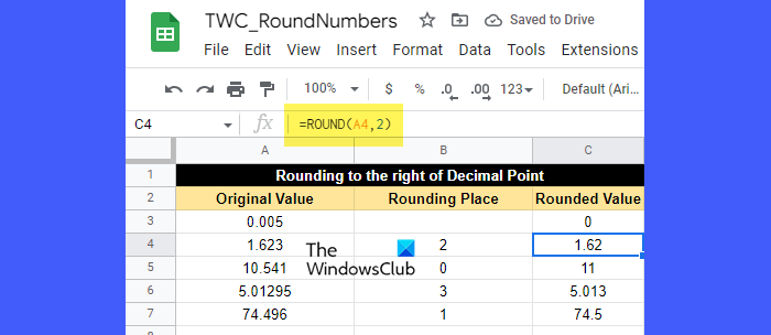
Suppose we have a spreadsheet with some sample data as shown in the above image. The first column lists some fractional figures that need to be rounded off to the number of places specified in the second column. To round these figures, we may use the ROUND function as follows:
Place the cursor in cell C3 and type the following function:
=ROUND(A3)
Since the number of decimal places to which the number needs to be rounded is not specified for cell A3, it will take the default value (0). This means there is no rounding digit, or in other words, the number needs to be rounded off to the nearest integer. Now since the digit to the right of the decimal point is 0 which is less than 5, the number to the left of the decimal point is left unchanged. So the resultant value will be 0, as displayed in cell C3.
For the next value (cell A4), the rounding place is 2. So the number needs to be rounded off to 2 decimal places. So the rounding digit is 2. The digit to the right of the rounding digit is 3, which is less than 5. So the rounding digit will be left unchanged. Therefore, the resultant rounded value will be 1.62, as shown in cell C4.
For the next value (cell A5), the rounding place is 0. Again, the number will be rounded off to the nearest integer which is 11, as displayed in cell C5. Here, since the digit to the right of the decimal point is equal to 5, the digit to the left is raised by 1.
Now for the next 2 values (in cells A6 and A7) you can easily determine how the ROUND function is rounding the values.
B] Round numbers to the left of the decimal point
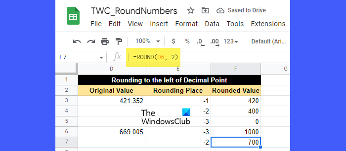
Suppose you need to round the number to the left of the decimal point instead of the right. For that, you need to pass a negative value in the places argument.
A negative value in the places argument will remove all the digits to the right of the decimal point and round the number to the left of the decimal point to the nearest tens, hundreds, thousands, and so on.
For example, look at the above image. We have passed negative values as places in the ROUND function. Here,
- -1 will round the number to the left of the decimal point to the nearest tens.
- -2 will round the number to the left of the decimal point to the nearest hundreds.
- -3 will round the number to the left of the decimal point to the nearest thousands, and so on.
Following this, the number in cell D3 (421.352) becomes 420 when rounded to the nearest tens, becomes 400 when rounded to the nearest hundreds, and becomes 0 when rounded to the nearest thousands.
Similarly, the number in cell D6 (669.005) becomes 1000 when rounded to the nearest thousands and becomes 700 when rounded to the nearest hundreds.
2] Round numbers using the ROUNDUP function
The ROUNDUP function works just like the ROUND function except that it always rounds the number upwards. The syntax of the ROUNDUP function is:
ROUNDUP(value, [places])
- Where value is the number that needs to be rounded upward, and
- [places] refers to the number of decimal places to which the number should be rounded. It is an optional argument and its default value is zero (0). If a negative value is passed in the places argument, the number to the left of the decimal point is rounded upward.
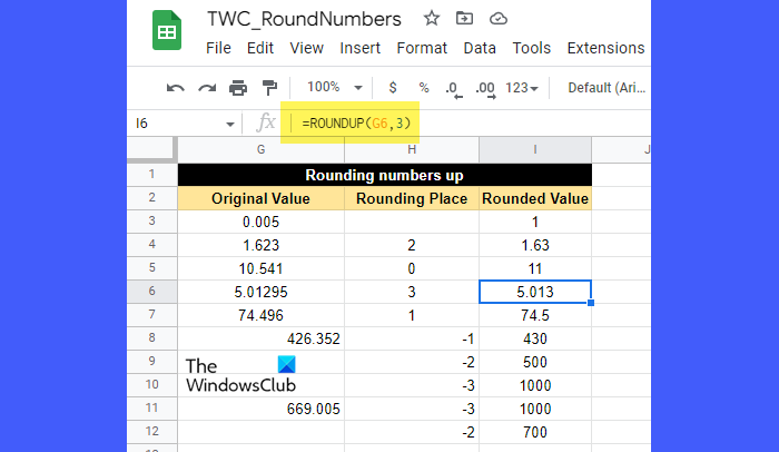
Now have a look at the above image. As you may see, all the numbers have been rounded upward to a certain number of decimal places either to the right of the decimal point or to the left of the decimal point, depending on whether the value of the places argument is positive or negative.
For example, the value in cell G4 (1.623) has been rounded up to 2 decimal places. Here, the rounding place is 2, which is digit 2, and the digit next to 2 is 3, which is less than 5. Still, since this is a ROUNDUP function, the resultant value will be 1.63 and not 1.62.
Similarly, the value in cell G8 (426.352) becomes 430 (not 420) when rounded up to the nearest tens.
3] Round numbers using the ROUNDDOWN function
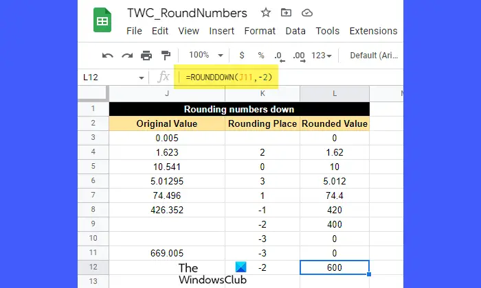
The ROUNDDOWN function also works like the ROUND function except that it always rounds the number downwards.
The syntax of the ROUNDDOWN function is:
ROUNDDOWN (value, [places])
- Where value is the number that needs to be rounded downwards, and
- [places] refers to the number of decimal places to which the number should be rounded. It is an optional argument and takes the value zero (0) if not specified by the user. The number to the left of the decimal point is rounded downward if a negative value is passed in the places argument.
Now have a look at the above image. Looking at the figures, you may easily understand how the ROUNDDOWN function is rounding the numbers down to a certain number of decimal places. The numbers are rounded either to the right of the decimal point or to the left of the decimal point based on the value of the places argument (positive or negative).
For example, the value in cell J7 (74.496) has been rounded down to 1 decimal place. Here the rounding place is 1, which is digit 4. The digit to the right of 4 is 9, which is greater than 5. Still, the rounded value will be 74.4 and not 74.5, since the ROUNDDOWN function has been applied to the cell value.
4] Round numbers using the MROUND function
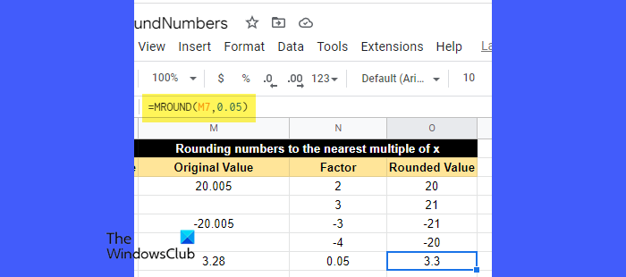
The MROUND function rounds a number to the closest multiple of another number, such as 2, 3, 5, etc.
The syntax of the MROUND function is:
MROUND(value,factor)
- Where value is the number that needs to be rounded, and
- factor is the number whose multiple becomes the closest number to which the given number should be rounded.
Notes:
- While using the MROUND function, you can pass a negative value in the factor argument only if the value argument is also negative.
- Both value and factor arguments can be non-integral.
- If 0 is passed in the factor argument, MROUND function will return 0.
- If 2 multiples of factor are equally nearest to the value, multiple with the higher absolute value will be returned.
To understand this, have a look at the above image. The value in cell M7 (3.28) has been rounded to 3.3. Here, the factor value is 0.05. If we keep on multiplying the factor with 1, 2, 3 and so on, we will find the following numbers nearest to 3.28:
0.05 x 64 = 3.2
0.05 x 65 = 3.25
0.05 x 66 = 3.3
0.05x 67 = 3.35
Out of all these, the closest is 3.3. So the MROUND function has returned 3.3 as a result.
5] Round numbers using the INT function
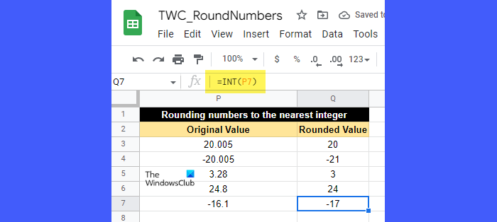
The INT function is used to round a decimal number downwards. It always rounds the number down to the nearest integer which is less than or equal to it.
The syntax of the INT function is:
INT(value)
- Where value is the number that needs to be rounded off.
To understand this, have a look at the above image. The value in cell P6 (24.8) has been rounded to 24, which is the nearest integer lesser than 24.8. Similarly, the value in cell P7 (-16.1) has been rounded to -17, which is the nearest integer lesser than -16.1.
The main difference between the INT function and the ROUNDDOWN function is that the INT function rounds the value of a given number downwards, whereas the ROUNDDOWN function rounds the ‘absolute’ value of a given number downwards. So if we apply the ROUNDDOWN function to cell P7, the result will be -16, not -17.
6] Round numbers using the FLOOR function
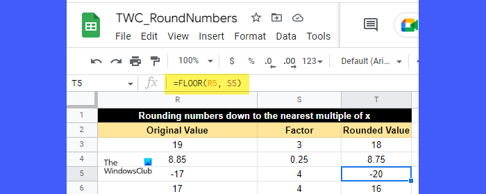
The FLOOR function rounds a given number down to the closest multiple of another number.
The syntax of the FLOOR function is:
FLOOR(value, [factor])
- Where value is the number that needs to be rounded, and
- factor is the number (positive only) whose multiple is the closest number to which the value should be rounded. It is an optional argument and its default value is 1.
To understand the FLOOR function, have a look at the above image. The value in cell R5 (-17) has been rounded down to -20, which is a multiple of 4, closest to -17. Similarly, the value in cell R3 (19) has been rounded down to 18, which is a multiple of 3 closest to 19.
Also Read: How to Highlight Duplicates in Google Sheets.
7] Round numbers using the CEILING function
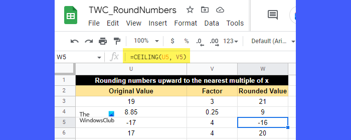
The CEILING function rounds a given number upward to the closest multiple of another number.
The syntax of the CEILING function is:
CEILING(value, [factor])
- Where value is the number that needs to be rounded, and
- factor is the number (positive or negative) whose multiple is the closest number to which the value should be rounded. It is an optional argument that takes the value 1 if not specified by the user.
If the value is positive, the factor must also be positive. But if the value is negative, the factor may either be positive or negative to determine in which direction the values should be rounded.
For example, look at the above image. The value in cell U5 (-17) has been rounded upward to -16, which is a multiple of 4 closest to -17. Similarly, the value in cell U3 (19) has been rounded upward to 21, which is a multiple of 3 closest to 19.
So this winds up how you may round numbers in Google Sheets. Hope you find this useful.
Read Next: How to stop Excel from rounding numbers.
Leave a Reply