In this tutorial, we will show a simple trick to show charts with hidden data in Excel.
Microsoft Excel is quite useful for analyzing trends and patterns in large data, It is easy to lay, reformat, and rearrange data, process data, and analyze charts and graphs. Using charts in Excel is very important to some people, especially if they want to show a graphical representation of their data. Excel contains features that assist people in showing their information graphically so that their audience can easily understand it. A person would use charts to showcase how many sales the company makes annually or how many scores students might get on a test. In Excel, people can even customize their charts by changing the color or rearranging the data position within the chart.

How to show Charts with Hidden Data Cells in Excel
When data is hidden in your table, Excel does not show that information in the chart. Follow the steps below to show charts with hidden data cells in Excel.
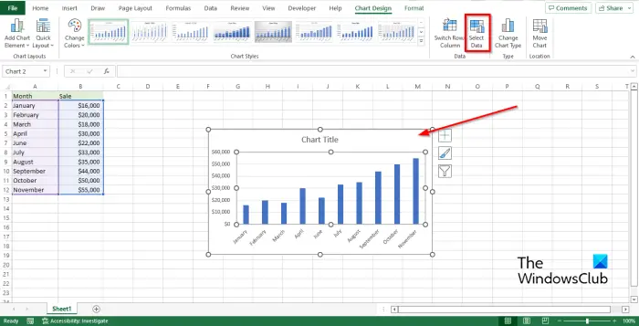
- Select the chart, then click the Chart Design tab.
- Click the Select Data button.
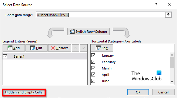
- Click the Hidden and empty cells button.
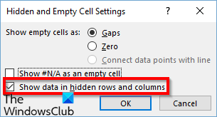
- Click the Show data in hidden rows and columns check box.
- Click OK for both dialog boxes.
In this tutorial, you will notice that the data for May is hidden.

Select the chart, then click the Chart Design tab.
Click the Select Data button in the Data group. The Select Data feature changes the data range included in the chart.
A Select Data Source dialog box will open.

Click the Hidden and empty cells button.
A Hidden and empty cells settings dialog box will open.

Click the Show data in hidden rows and columns check box, then click OK for both dialog boxes.

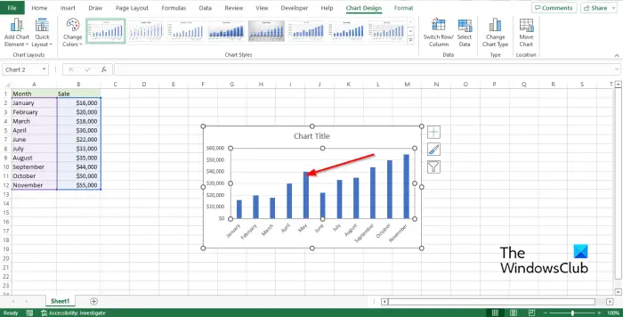
You will notice that the May information that was missing is now shown in the chart.
We hope you understand how to show charts with hidden data in Excel.
How do I remove extra data from Excel chart?
Follow the steps below to remove extra data from an Excel Chart.
- Click anywhere on your chart.
- Click the Filter button next to the chart.
- On the Values tab, check or uncheck the series or categories that you want to change.
- Then click Apply.
READ: How to create a Lollipop Chart in Excel
How do I get a chart to ignore blank cells?
Follow the steps below on how to ignore blank cells in Excel:
- Select a blank cell next to the values that you want to use to create the chart and type the formula
=IF(ISBLANK(C2), #N/A, C2). C2 is the cell that you will use and drag the auto fill handle down to the cells you need to apply this formula. - Then click the Insert tab and select a Chart from the chart group.
- After the chart is inserted, you will notice that Excel will ignore the blank cells in the chart.
Leave a Reply