If you are wondering how to use the Excel FILTER function with multiple criteria, here’s a tutorial to guide you through the steps and ensure you can efficiently filter and sort your data.
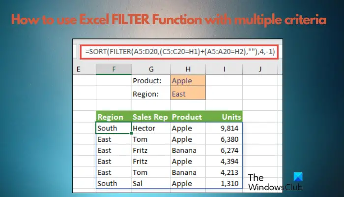
The FILTER function in Excel is a powerful tool that allows you to extract specific data from a range, of data lists or an array based on multiple criteria. By using this function, you can easily filter and display only the information you need, saving you time and effort in searching and organizing your data.
What Is the FILTER Function in Excel?
The basic syntax to filter a range, list, or array of data using single or multiple criteria is as follows:
=FILTER(array, include, [if_empty])
So, if you want to extract specific data from a large set of data, for example, from 1000 rows, this Filter Function formula makes things easier. Previously, we would use only the drop-down lists with checkboxes to filter data, but it would not help with complex criteria.
That said, there are three input arguments for the Excel Filter function:
- Array: The range of cells that you want to filter.
- Include: The criterion to filter the data which should be in the form of a boolean equation. For example, the input should be yes or no using symbols like =, >, <, etc.
- [If_empty]: This optional input (“ ” or N/A or No Results) instructs Excel to place a value or string of text when the filter returns an empty table.
Using the basic Excel filter function formula
Before we explain how to use the Excel filter function with multiple criteria, it’s important to understand how the Excel filter function formula works.
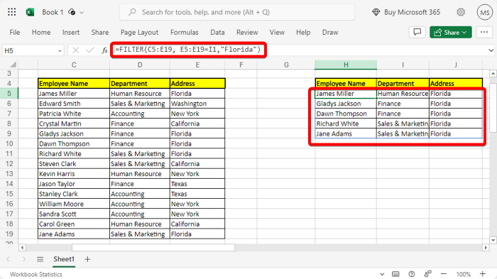
Here’s an example of a basic Excel filter function formula, for example, filter how many employees stay in Florida (refer to the table):
=FILTER(C5:E19, E5:E19=I1,"Florida")
The formula extracts the result in the cell range (H4:J9) without altering the original data.
Alternatively, you can also use the built-in Filter function to make things easier. Simply select the data range, go to Home, and click on the Sort & Filter icon.
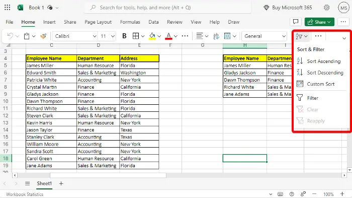
Select Filter from the menu to add drop-downs to the selected range.
Next, go to the Address column, select the drop-down, uncheck Select All, and select only Florida.
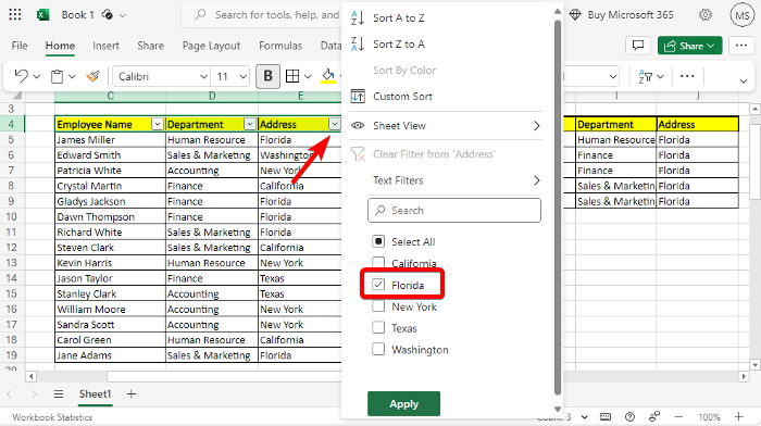
The cells will now show only the names of the people from Florida and their respective Departments.
But if you encounter any SPILL errors in Excel, refer to our linked post for the solutions.
How to use the Excel filter function with multiple criteria
Now that you understand how to use the basic filter function in Excel, here’s a Microsoft Excel tutorial on using the Filter function with multiple criteria.
To use more than one criterion for data filtering, you can perform either the AND or OR operation.
1] Using the AND operation with multiple criteria
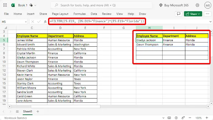
While the AND function requires all the criteria to be True to have the row included in the filter result, the OR function needs at least one of the criteria to be True to have the row included in the filter result.
So, here’s an example that shows how to use the AND logical function in the Excel FILTER function to pull up data from a specific cell range with two criteria:
=FILTER(C5:E19, (D5:D19="Finance")*(E5:E19="Florida"))
This will extract how many Finance department employees are from Florida.
Read: How to use Slicers to filter Data in Excel
2] Using the OR operation with multiple criteria
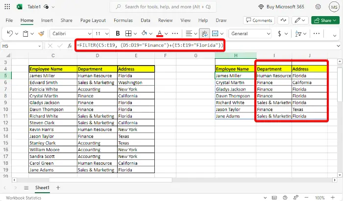
The OR operation is fulfilled when any one or more than one criteria are fulfilled. So, for example, if you want to find out how many employees are from Accounting OR Finance, all you need to do is use the above formula and replace the * operator with + as demonstrated below:
=FILTER(C5:E19, (D5:D19="Finance")+(E5:E19="Florida"))
That’s it, and it should return the two results in two separate columns.
But if you prefer using Microsoft Access, here’s how you can sort and filter records in Access.
Read: Excel filter not working properly
How do you put multiple conditions in a filter?
To use a filter with multiple conditions, you can combine them using logical operators like AND and OR. For example, in a spreadsheet, you might use the formula, =FILTER(range, (condition1) + (condition2), “”) for the OR operator. Or, you can use the formula =FILTER(range, (condition1) * (condition2), “”) for the AND operator. Also, make sure that your conditions are appropriately set for accurate results.
How to do multiple selections in Excel filter?
To do a multiple selection in Excel filter, click the drop-down arrow in the column header. Then select Filter by Color or Text Filters to specify your criteria. To select non-contiguous items, hold Ctrl and click each item. For continuous items, click the first item, hold Shift, and click the last item. This effectively applies multiple filters for advanced data sorting.
Leave a Reply