The CHOOSE function in Microsoft Excel is a Lookup and Reference function, and its purpose is to choose a value from a list of values. The CHOOSE function formula is CHOOSE(index_num, value 1, [value 2]..).
- Index_num: The value to choose, this is required.
- Value1: The first value to choose. It is required.
- Value 2: the second value to choose. It is optional.
How to use the CHOOSE function in Excel
Open Microsoft Excel.
Create a table or open an existing table.
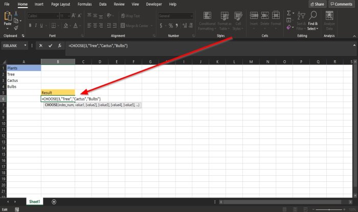
In this tutorial, we have a table of plants; we want to find which value is at number three.
In the cell where you want to place the result, enter:
=CHOOSE(3, "Tree," "Cactus," "Bulbs")
The number three is the Index_num and the position of the plant.
Tree, Cactus, and Bulbs are the Values.
Then press Enter on the Keyboard.
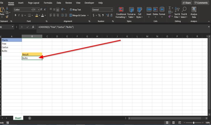
You will see the result.
There are two other methods of using the CHOOSE function.
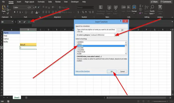
Method one is to click the fx button on top of the worksheet.
A Select Function dialog box will pop up.
In the Select a Function dialog box, click the drop-down arrow and select Lookup and Reference in the Select a Category section.
In the Select a Function list, select CHOOSE from the list.
Then OK.
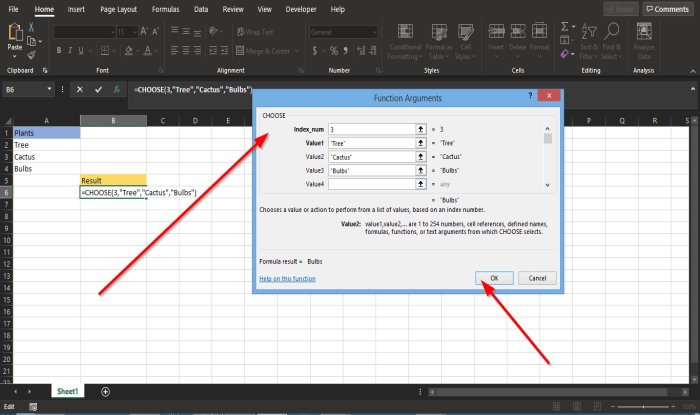
A Function Arguments dialog box will pop up.
In the Index_num section, enter the number Three into the entry box.
In the Value one section, enter Tree into the entry box.
In Value two, enter Cactus into the entry box.
In Value three, enter Bulb into the entry box.
Then OK.
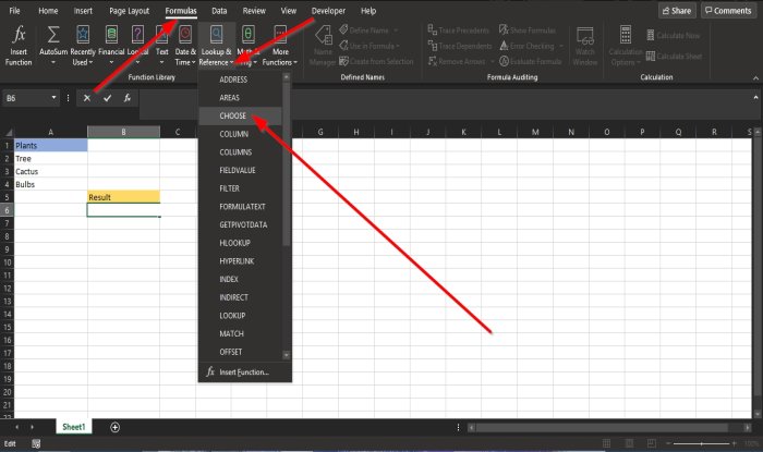
Method two is to click the Formulas tab and click the Lookup and Reference button in the Function Library group.
In the drop-down list, select CHOOSE.
A Function Arguments dialog box will open.
Follow method one to see the steps.
Then click OK.
We hope this tutorial helps you understand how to use the CHOOSE function in Excel; if you have questions about the tutorial, let us know in the comments.
TIP: This post will help you if the Auto Fill options are not showing in Excel.