The Hyperlink function creates shortcuts that leap to another location. The Hyperlink function can create links to workbooks, documents stored on a network server, intranet, or the internet when we click on a cell with a Hyperlink function. Excel will open the document specified or go to the location listed. The formula for the Hyperlink function is: HYPERLINK (link_location, [friendly_name]).
The syntax for the Hyperlink Function
- Link_location: The path and file name to be open, it is required.
- Friendly_name: The link text or number displayed in the cell. Friendly_name is optional.
This article will explain how to create a hyperlink in an excel worksheet using a Hyperlink function.
How to use Excel Hyperlink Function
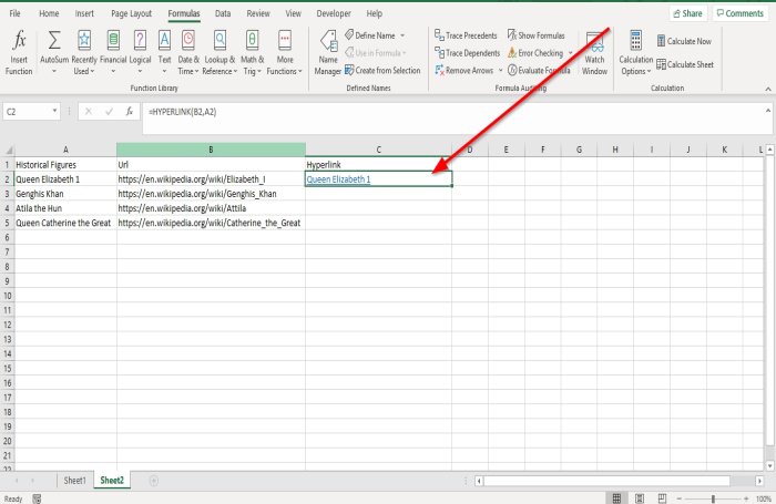
In this tutorial, we are going to create a hyperlink for some historical figures in the table.
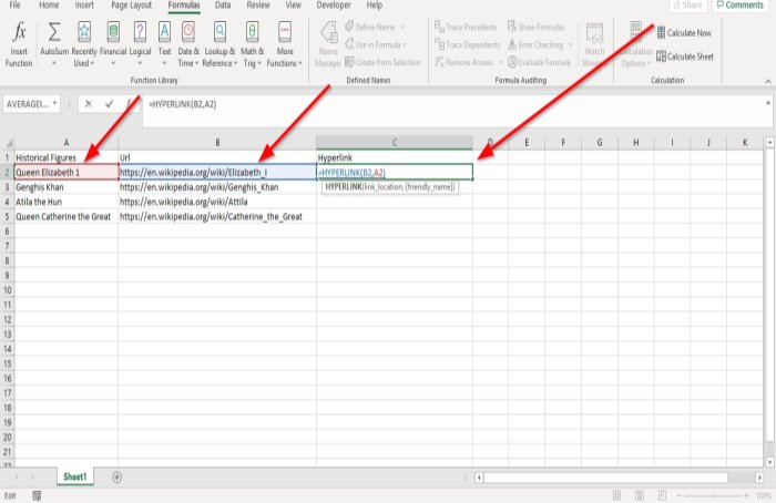
Click the cell where you want the result to be.
Type the formula =HYPERLINK then bracket.
We are going to enter Link_location. In the example (see in the image above) where you see the URL of the sites, type B2 because the site you want to link to is in the URL column.
Now enter the Friendly_name. The friendly name will be the data located in the historical figure column. Type A2, because we want to link the data in the URL and historical figures column together. Close bracket.
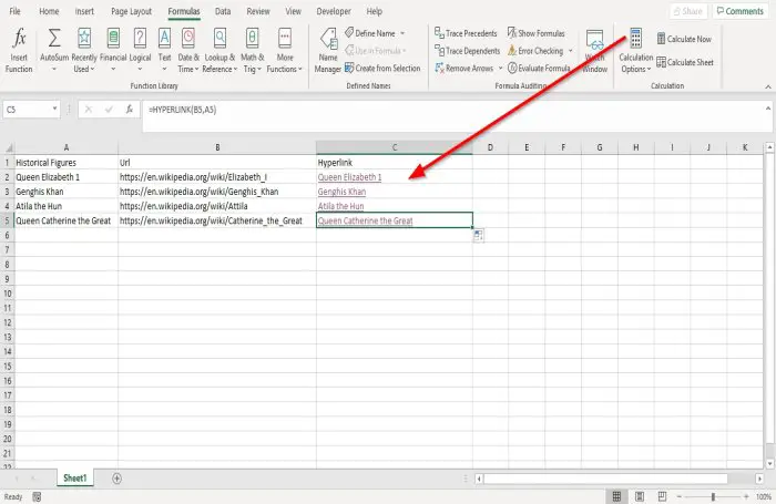
Press Enter you will see your result.
Suppose you want to see results for the other data using the Hyperlink function. Click the cell and drag it down.
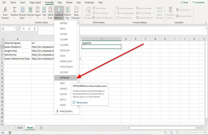
The other option is to go to Formula. In the Function Library group, click Lookup and Reference; in the drop-down menu, select Hyperlink. A Function Arguments dialog box will appear.
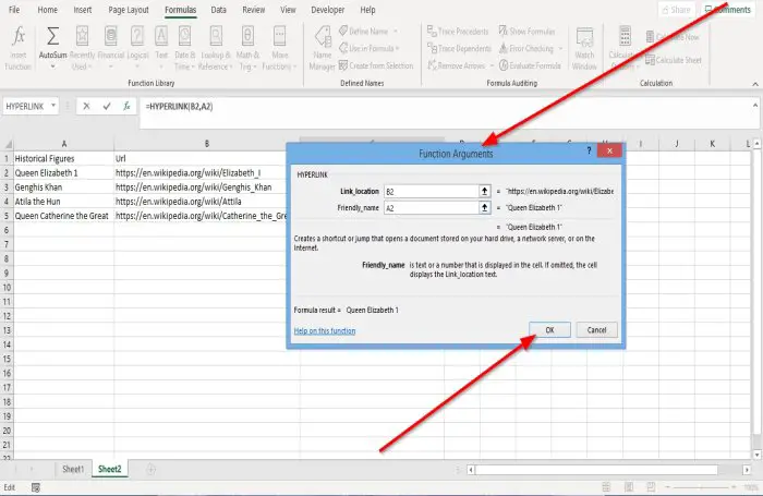
On the Function Arguments dialog box, where you see Link_location, type the cell B2 into the entry box.
Where you see Friendly_name, type the cell A2 into the entry box.
Click, OK; you will see the result.
I hope this helps.
Now read: How to use Hour, Minute, and Second Function in Excel.