The Mode function in Excel returns the most frequently repetitive value in an array or range of data. The formula for Mode function is Mode( number1, [number2,..]).

In Excel, Modes can be arrays, numbers, names, or suggestions that contain numbers. The Mode function ignores values such as text, logical values, or empty cells in an array or reference argument. Error-values and text that cannot be translated into numbers cause errors, and if the data set contains no duplicate data, the Mode will return to the #N/A error value.

In Microsoft Excel, the Mode function is classified as a compatibility function and recommends using the MODE.MULT and MODE.SNGL instead.

The Syntax for the Mode function

Number1: The number argument for which you want to calculate the Mode. It is required.
Number2: The Second number argument for which you want to calculate the Mode. It is optional.

How to use the Mode function in Excel

Open Microsoft Excel.

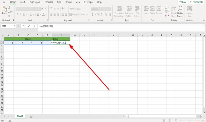
Create an Excel table with a few repetitive numbers.

Type into the cell where you want to place the result, =MODE(A2:E2).

A2:E2 is where the range of data is.

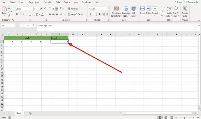
Then press the Enter key, you will see the result.

There is another method to use the Mode function.

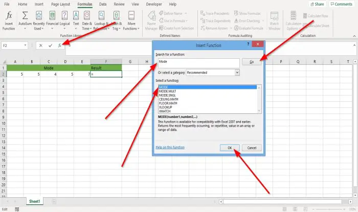
Click the fx button at the top of the excel worksheet.

An Insert Function dialog box will open.

Inside the Insert Function dialog box, at the Search Function box, type Mode into the box.

Then, click Go.

At the Select a Function section, click Mode in the list box.

Then. Click OK.

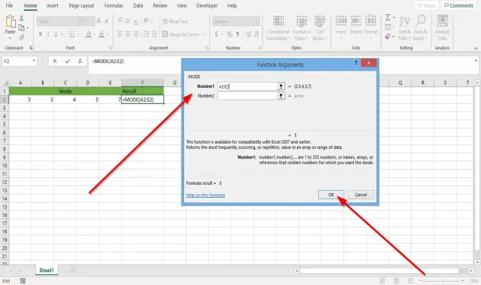
A Functions Arguments dialog box will appear.

Inside the Functions Arguments dialog box, where you see Number1, we type into the entry box A2:E2 because this is the range of cells where we want to find the Mode.

Number2 is optional.

Click OK, and you will see the result.

I hope this helps; if you have questions, please comment below.