How to split Data into Rows using Power Query

In this post, we will show you how to split Data into Rows using Power Query. While exporting data from other systems or sources, you may encounter situations when the data is stored in a format where multiple values are combined into a single cell.

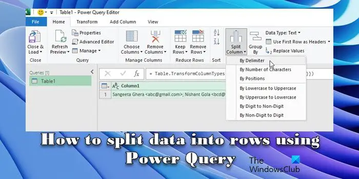
This could happen when users inadvertently enter multiple pieces of information into a single cell if they’re unfamiliar with Excel’s conventions, or when they copy/paste data from another source without proper formatting. Dealing with such data requires additional steps to extract and organize the information for analysis or reporting purposes.

How do you split data in Power Query?

Power Query transformations can assist in splitting data into distinct cells or rows, based on various factors such as delimiter, text patterns, and data types. You can split data by selecting the column containing the data you want to split and then using the ‘Split Column’ option from the ‘Transform’ tab in the Power Query Editor. In this post, we will see how to split data into rows using Power Query.

How to split Data into Rows using Power Query

To split data into rows using Power Query, you need to follow these steps:

Let us assume that our data consists of a string of text with delimiters (names and email addresses separated by a semicolon), as shown in the screenshot below.

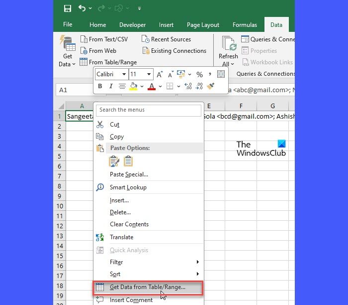
Right-click the cell that contains your data and select Get Data from Table/Range from the context menu.

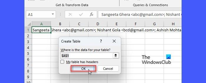
Click on OK in the Create Table popup, while ensuring that the ‘My table has headers’ option is unchecked. The data will open in the Power Query Editor.

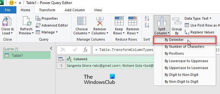
Split data into Rows by Delimeter

By default, Power Query will treat the entire cell content as a single value and load it as a single record with one column and one row. To split the data, go to the Split Column menu within the Home tab and select By Delimiter. This option allows you to split values in the selected column based on a specified delimiter. The rest of the options in the menu let you split column values based on other factors, such as a specified number of characters, positions, or transitions.

Once you click on ‘By Delimiter’, a Split Column by Delimiter window will appear. Select a delimiter (a character or sequence of characters that separate and distinguish individual values within your dataset) in the Select or enter delimiter dropdown. Since a semicolon separates the data values in our case, we have selected Semicolon from the dropdown menu, as shown in the screenshot below:

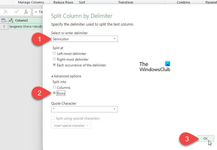
Next, click and expand the Advanced options and select Split into ‘Rows‘. Click OK to apply the changes.

Now Power Query will parse your data, split it at each occurrence of the semicolon, and place each entry in its own individual row.

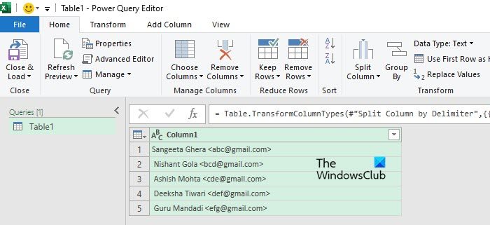
As you can see in the above screenshot, our data has been split nicely into multiple rows. Again, we will split the data to separate the names from the email addresses.

Split data into Columns by Delimeter

Click on the Split Column dropdown under the Transform section within the Home tab and select By Delimiter. The Split Column by Delimiter window will appear.

For Power Query to properly transform the data, you must correctly identify and specify the delimiter. For example, in our case, a less than sign (<) separates the names and the email addresses. So we will select Custom under the Select or enter delimiter dropdown and type the less than symbol (in most cases, Power Query will automatically try to figure out whether or not your data contains values separated by a delimiter and if so, what that delimiter is).

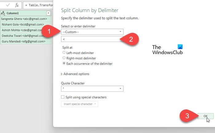
This time, we will not click on the ‘Advanced options’ dropdown since we want to leave the default value selected, which is Split into ‘Columns’. Click OK to apply the changes.

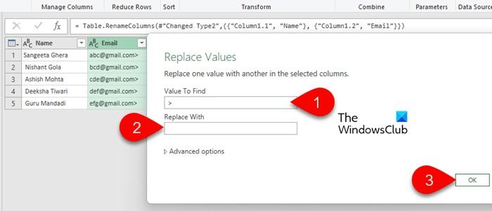
Power Query will transform your data and put the names and email addresses in individual columns, as shown in the screenshot below:

Note:

You may perform additional steps to remove blank spaces or extra characters from your data. For example, there’s a greater than symbol (>) that follows each email address in our case. To get rid of it, we will right-click on the column header and select Replace Values. Then replace ‘<‘ with nothing (enter ‘<‘ in the ‘Value To Find’ field and leave the ‘Replace With’ field blank).
You may give each column a descriptive name by double-clicking on its header.

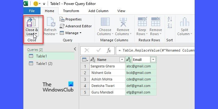
Once done, click the Close & Load button in the top-left corner of the Power Query Editor to export the data in a new Excel worksheet.

That’s it! I hope you find this useful.

Read: How to convert Columns to Rows in Excel with Formulas.

How do you turn columns into rows in Power Query?

Select the columns you want to turn into rows. Go to the Transform tab. Then go to the Unpivot Columns menu within the ‘Any Column’ group and select Unpivot Only Selected Columns. Power Query will transform the selected columns into rows and create two new columns, one for attribute names and one for their corresponding values. Rename columns if required and click on the Close & Load button to save changes to your data.