The SUMIF function purpose is to sum the values in a range that meets the criteria you specify or add a range based on a single criterion. SUMIF takes three arguments Range, Criteria, and Sum-range. Arguments are values that a function uses to perform operations or calculations in a formula.
The SUMIFS function adds all its arguments that meet multiple criteria. The orders of the SUMIFS function is different from the SUMIF function. In SUMIF, the Sum_ range is the third argument. In SUMIFS, the Sum_range is the first argument.
Difference between SUMIF and SUMIFS Syntax
SUMIF Syntax
- Range: The range of cells you want the function to calculate. The cells in range must be numbers, names, arrays, and references that contain numbers.
- Criteria: The condition or criteria you must look up for in the range provided in the first argument. The criteria are in the form of a text, number, and expression that identifies, which cells will be added.
- Sum_range: The range to be sum or cells to be added. The Sum_range is optional.
The formula is SUMIF (range, criteria, [sum_range]).
SUMIFS Syntax
- Sum_range: the range of cells to add.
- Criteria_range 1: The range of cells that is analyzed using criteria 1.
- Criteria 1: Determines the range of cells to add.
- Criteria_range2, criteria2: The additional ranges and their associated criteria. This argument is optional. The formula is
SUMIFS (sum_range, criteria_range1, criteria1 [criteria_range2, criteria2,..].
How to use the Excel SUMIF function
In this table, we want to calculate the number of mangoes sold.
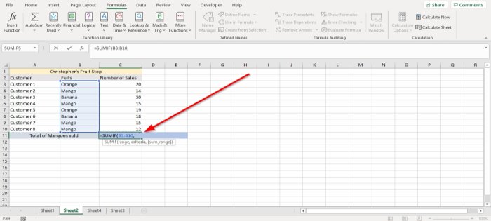
We are going to click the cell where we want to place the result.
Then type in the cell =SUMIF (
We are going to look for the Range. In this article, the Range is where you see the fruits because we want to find the number of mangoes sold.
Take the cursor and click on the cell B3 in the fruit column, then press the Ctrl, Shift, and the Down Arrow Key to highlight the data to B10 in the column or type B3:B10. You will see the Range of cells in the formula. Then add a comma.
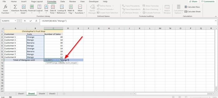
Then add the Criteria, which is Mango, because we want to find the sum of mangoes sold, then add a comma.
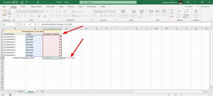
Add the Sum_range, the data located in the column labeled Number of Sales, that Displays the items purchased by each customer.
Click the cell of the first data in the Number of Sale columns. Press the Ctrl, Shift, and the Down Arrow Key to highlight the column’s data. Then add a bracket or type C3:C10.
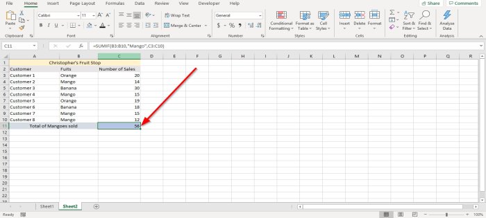
Press enter. You will see the result.
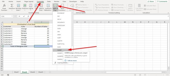
The other option is to go to the Formulas tab in the function and library group; click Math and Trig.
In the drop-down menu, select SUMIF. A function argument dialog box will appear.
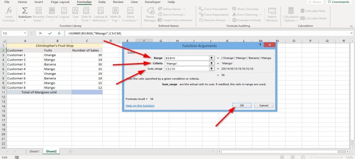
In the Range entry box, type the B3:B10.
In the Criteria entry box, type Mango because we want to find how many mangoes were Purchased.
In Sum_range entry box type C5:C10, this column is where the number of items purchased or located.
Press OK. You will see the result.
How to use the SUMIFS function in Excel
In this tutorial, we want to add the total number of sales of mangoes we made from, say, Kevin Sahadeo.
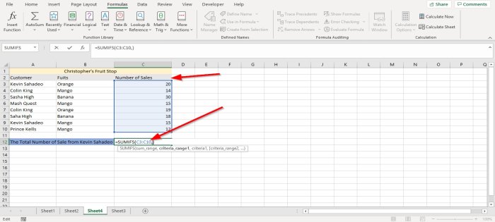
Click the cell where you want the result to be. Type, =SUMIFS () in the cell.
In the SUMIFS function, we will add the Sum_range first, which is the data in the Number of Sales columns, which specify how many items were purchased by each customer.
Type the cell C3:C10 or click on C3 and press the Ctrl, Shift, and Down Arrow Key to highlight down to C10, then add a comma.
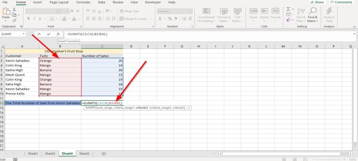
Add the Criteria range 1. Click the first data in the fruits column and enter the cells B3:B10 or Ctrl, Shift and Down arrow key to highlight the cells.
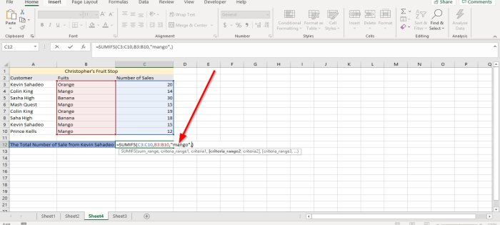
Type Mango as Criteria.
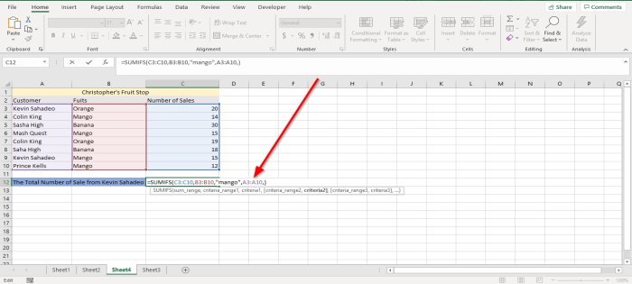
Now I am going to add the Second Criteria Range. Go to the Customer column and click on the first data in the table and Ctrl, Shift, and Down Arrow Key to highlight or type A3:A10, the comma.
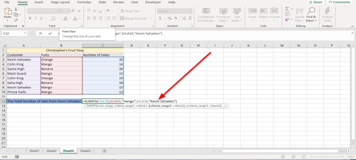
We are going to add the Second Criteria, which is Kevin Sahadeo. Ensure you type it the exact spelling in the formula and use the full name. Press Enter you will see the result.
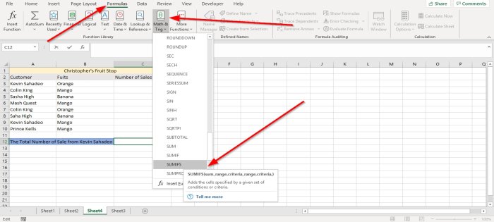
The other option is to click on the Formulas tab in the function library group, select Math and Trig in the drop-down menu, select SUMIFS. A function argument dialog box will appear.
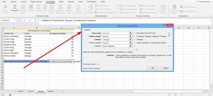
In the Sum_range entry box, type C3:C10 because this is the number of sales we want to add up.
In the Criteria_ range entry box type B3:B10 because this is the range where the fruit, we are looking for is.
In the Criteria entry box, type Mango because we want to find how many mangoes Kevin Sahadeo purchased.
In the Criteria_ Range 2 entry box type A3:A10, because this is the second range you are looking up, where the name Kevin Sahadeo is.
In the Criteria 2 entry box, type Kevin Sahadeo because we want to find out how many mangoes this person purchases.

Then click OK. You will see the result.
I hope you find the post useful.
Read next: How to create a Pivot Table and Pivot Chart in Excel.
Leave a Reply