If you are a regular Microsoft Excel user but not quite familiar with Power Query Add-in for Excel, then this post will acquaint you and help you get started with it. Any advanced Excel user faces the challenge of analyzing or creating reports with PivotTables and PivotCharts as they lack expertise in this domain and often show static tabular data or summaries. Though it is easy to use this table for quick data entry, it is difficult to start data analysis on such a table or convert it into PivotTable and shape it to meet your analysis needs.
Look no further, with Power Query technology in Excel; you can change this. The new capability added to Excel allows you to unpivot static tables, i.e., access your tables, perform a transformation, and create a PivotTable from the transformed data in Excel.
How to Unpivot Data in Excel
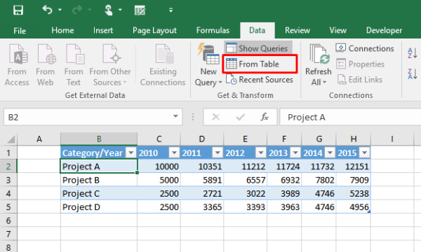
Consider you have an Excel workbook that is dedicated to manual data entry to track the number of hours you expend energy on a single relevant project.

Analyzing this data can be a daunting task. You wish if you could just create charts on this data. Fortunately, through the new Get & Transform section in the Data tab of Excel, you could complete the task. To do so,
Simply select any cell inside an existing table or range and in the Get & Transform section, click From Table.

You will see a preview of your data inside the Query Editor window. Under this window, you can start transforming your data. Each change you make is recorded as a transformation step that is saved in your workbook. All the steps are kept as a sequence and can be performed whenever you refresh your data.
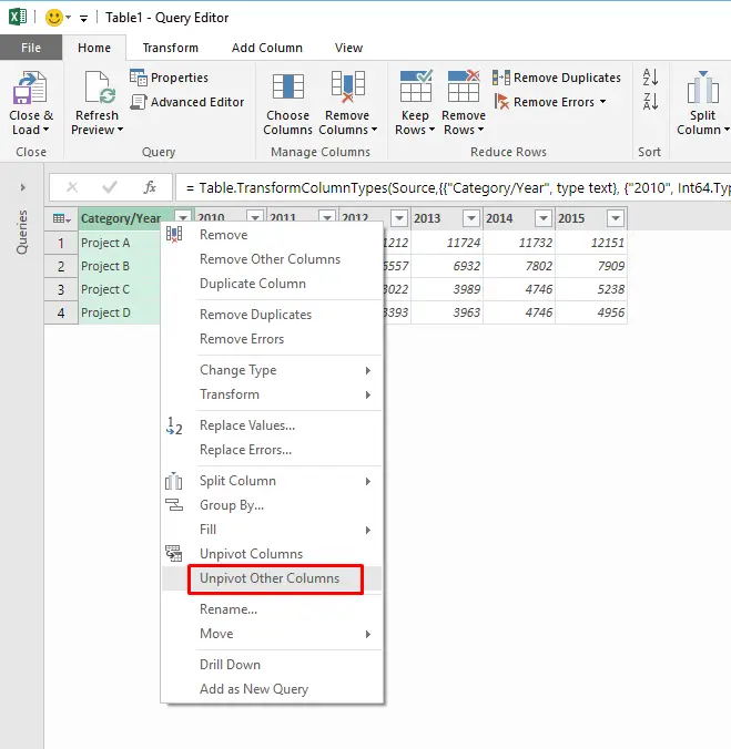
In the Query Editor, you will usually need the help of the Unpivot transformation to change your table into a format that can be used by PivotTable.
As you can notice in the example below, I can select the first column that includes project names and click Unpivot Other Columns to transform my data from columns of Project Name / 2010 / 2011 / 2012… to the desired column structure of Project / Year / Duration.

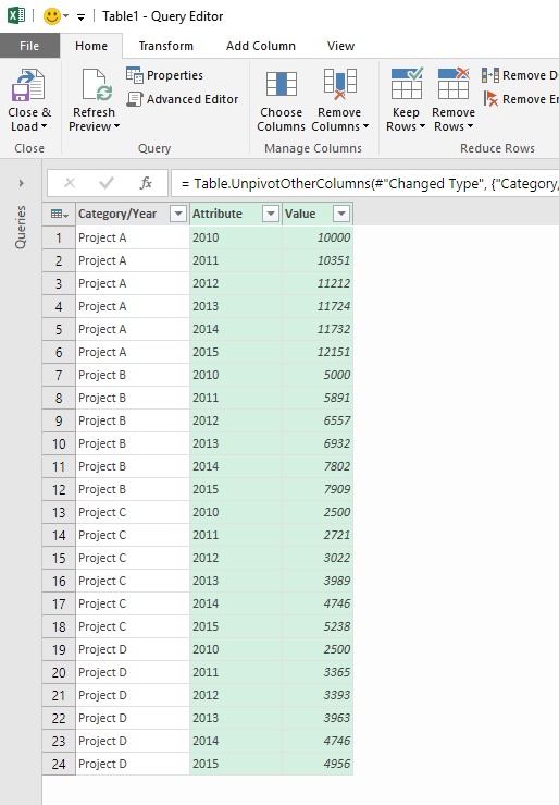
And here’s what you will find as the results in the Query Editor:

I can now rename the columns to Project, Year and Duration inside the Query Editor and then load the data into a PivotTable or PivotChart.
I hope this helps.
Now read: How to Display or Format Number as Currency in Excel.