How to use DSUM function in Excel

The DSUM Function in Excel sums up a column in a table based on multiple criteria that you specify. The DSUM function is a Database function. The formula for the DSUM Function is (database, field, criteria)

The syntax for the DSUM Function

• Database: The cells that make up the Database
• Fields: reveals which column is to be used in the function
• Criteria: The criteria range you specify

How to use DSUM function in Excel

Open Microsoft Excel.

Open an existing table or create a new table.

In this tutorial, we want to find Barbie Extra Dolls sales from the ninth to sixteenth of January.

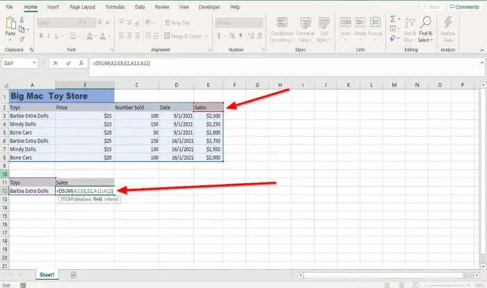
Below the table, you have created. Create a mini table of the criteria you are going to look for. In this tutorial, we create a mini table with the fields, toy, and sales.

In the Field “Toy,” we will put the criteria we are going to look for, that is “Barbie Extra Doll.”

We will place the cell’s cursor under the Field “Sales” and type in the cell =DSUM, then bracket.

Inside the bracket, type the Database, which is the table (A2:E8).

• Place a comma and type the Field, which is the cell’s field name (E2).
• Then place another comma and type the Criteria. The Criteria is what you are looking for (A11:A12).

The formula should look like this =DSUM (A2:E8, E2, A11:A12).

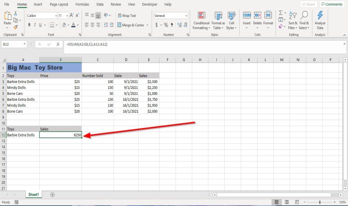
Press Enter you will see the results.

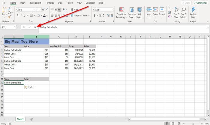
The other option is to click Insert Function (fx)

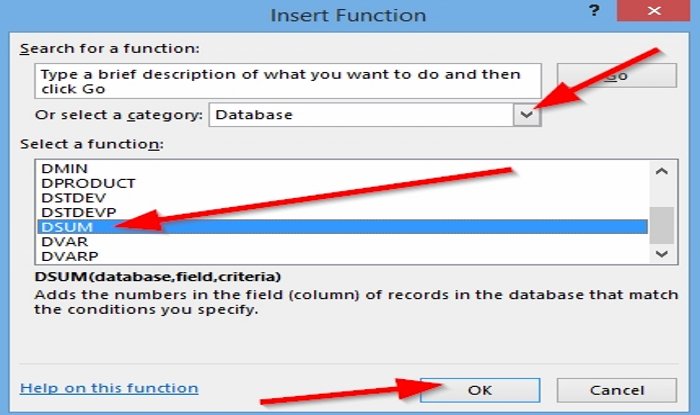
An Insert Function dialog box will appear.

In the dialog box, select the category Database.

Select the function DSUM, then press OK.

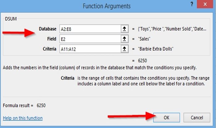
A Function Arguments Dialog box will pop up.

In the Functions Argument dialog box, type in the Database entry box A2:E8.

In the Field’s entry box, type E2 or “Sales.”

In the Criteria entry box, type A11:A12 and press OK.

I hope this is helpful; if you have a question, please comment below.

Read next: How to Use EDATE and EOMONTH Function in Excel.