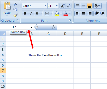
Many of us use Microsoft Excel to calculate the budget or do some additions and subtractions. We also know that it supports Macros which helps us to automate our tasks. An Excel sheet is no stranger to us and does not require any introduction. But how many of you know there is a box called Name Box in Excel sheet that we use daily?
Yes, I am talking about the box at the top left and under the ribbon. We generally think it is just the normal box that gives reference to the active cell. But there is a lot to know about this, and we need to know the use of Excel Name Box.
What is the Name Box function in Microsoft Excel?
The Name Box function in Microsoft Excel displays the cell currently selected in the spreadsheet. It is located to the left of the formula bar. If a name is defined for a selected cell, the Name Box displays the name of the cell. You can use the Name Box to define names for cells, ranges, constants, and formulas.
How to use Name Box in Excel
Uses of Name Box in Excel
I will take you through some tips and tricks that this Excel Name Box can implement.
Quickly go to the specific cell
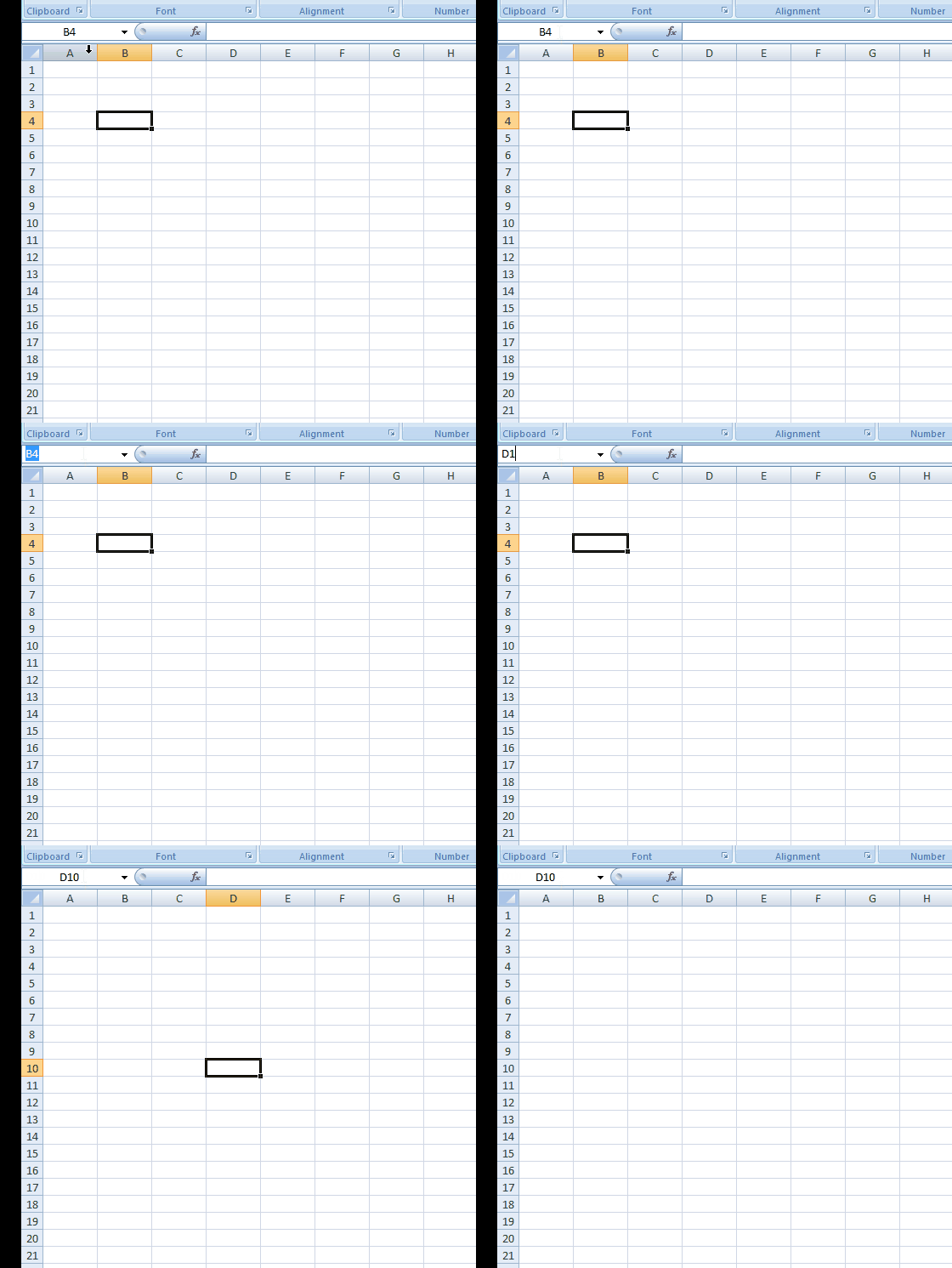
If you want to go to a specific cell, then you can type the address of that cell in this Name Box. For example, if you want to go to D10, then type D10 into the Name Box, and that particular cell gets active.
Select and Move to a specific range of cells
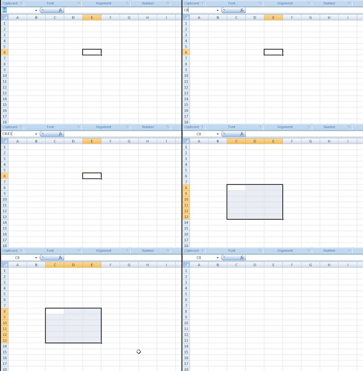
If you want to select and move to a specific range of cells, then you can use Excel Name Box. For example, if you want to select a range from C8 to E13, you can type C8:E13 in the Name Box and hit Enter. Even if you are at another location, say Q10, you will return to the selected range as specified in the Excel Name Box.
Select a particular range from an active cell
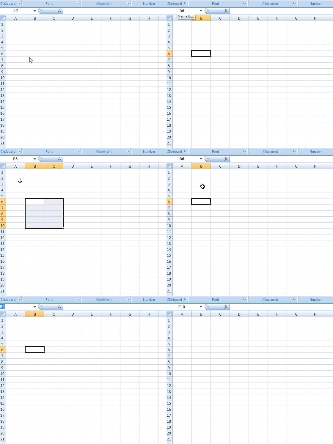
If the active cell is B6 and you type C10 in the Name Box, press and hold the Shift key of the keyboard and hit enter. You can see that range B6:C10 will be selected. Try pressing and holding the Ctrl key, and you see that only cells B6 and C10 will be selected and not the range. Identify the difference between them.
Select Multiple Particular Cells
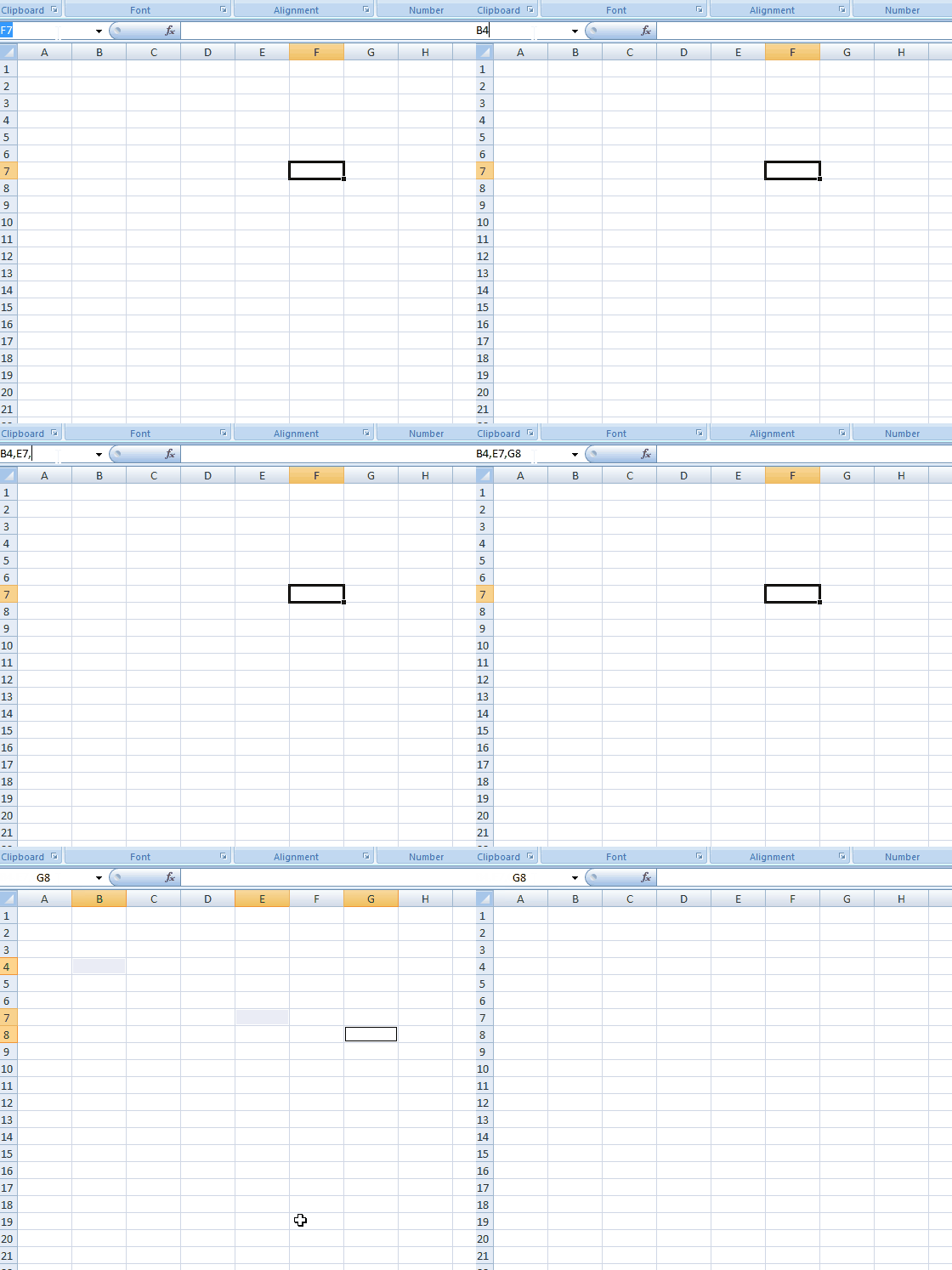
Type B4, E7, and G8 in the Name Box and hit enter. You see that all three calls are selected. You can try with A10, B17, and E5 and let us know. Note that the commas are used without any space.
Select Multiple Particular Ranges
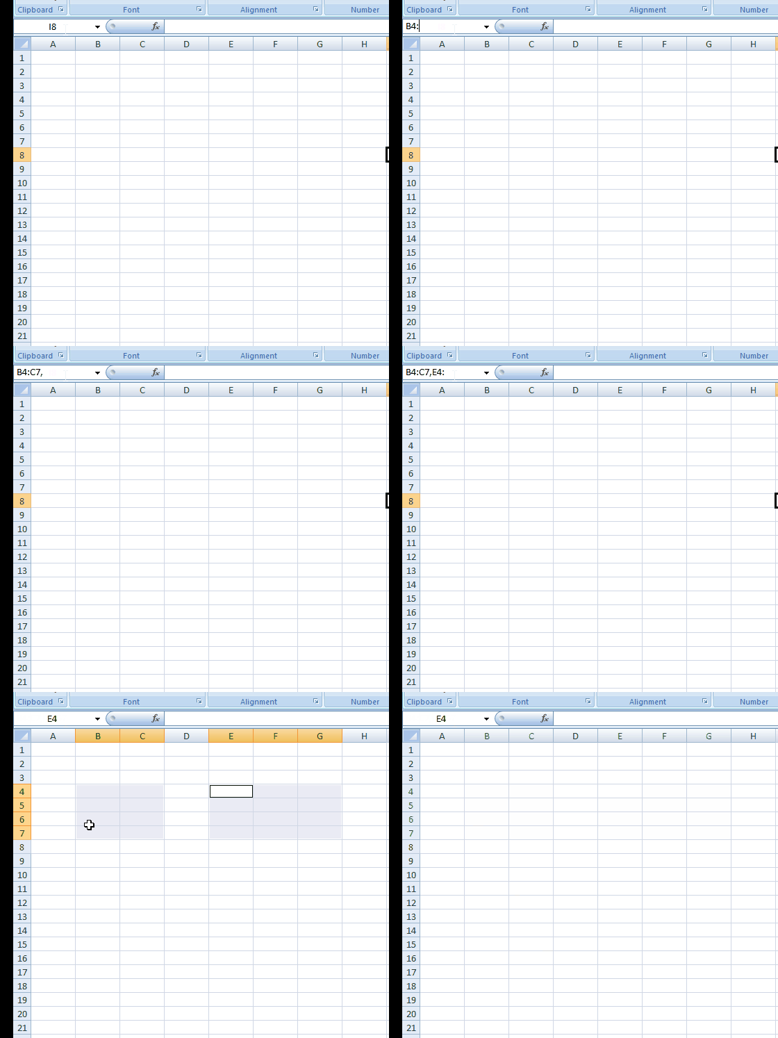
Type B4:C7 and E4:G7 in the Name Box and hit Enter. You see that two specific ranges, B4 through C7 and E4 through G7, got selected. Identify the colon and comma regarding the placement.
To select entire Column(s)
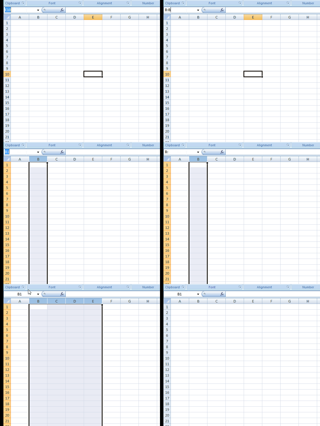
Type B:B in the Name Box and enter to see that the entire column B has been selected. Try typing B:E, and you see that all columns from B to E will be selected completely.
To select entire Rows(s)
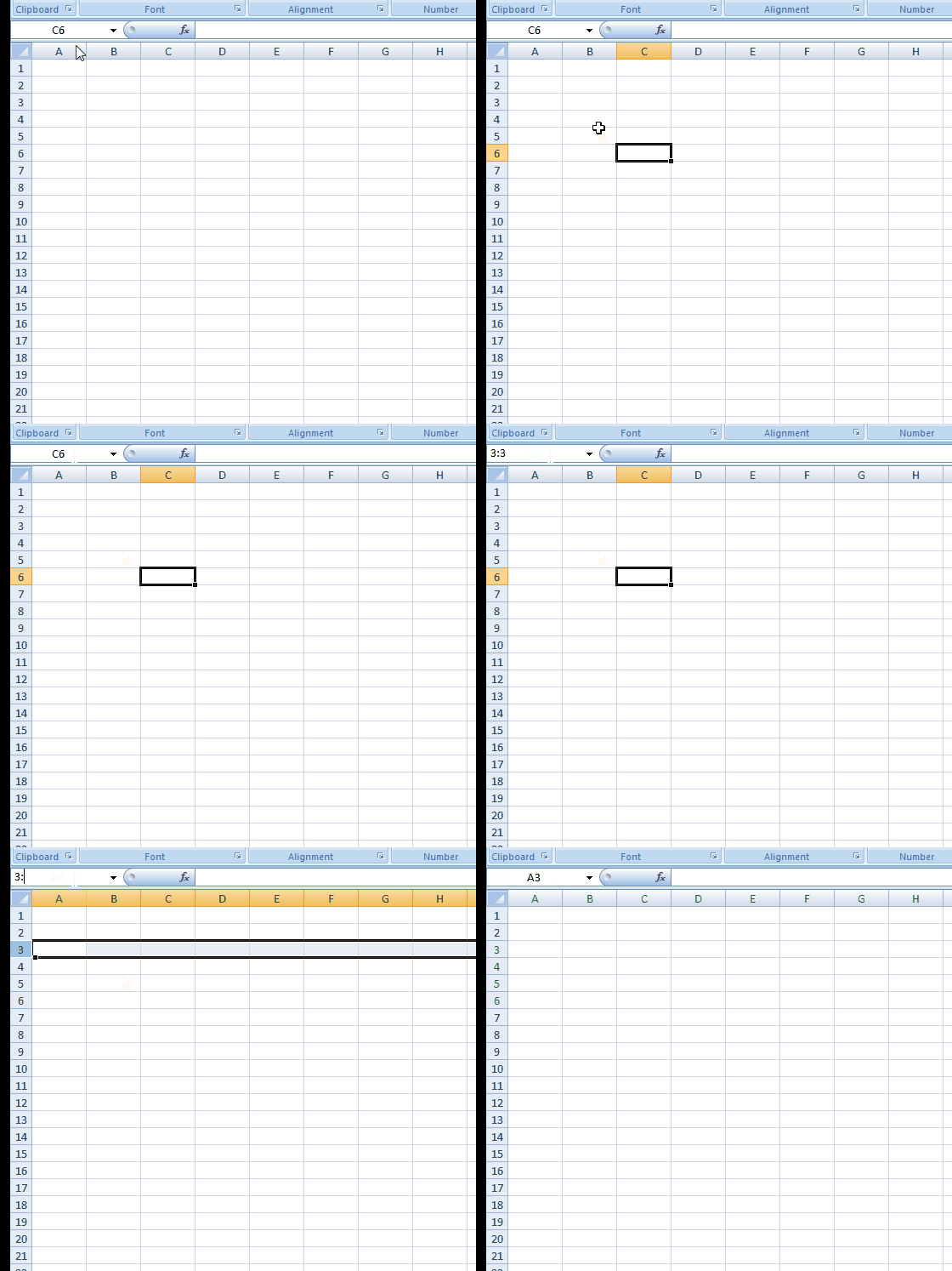
Type 3:3 in the Name Box, and you will see that row 3 is selected. Type 3:6, and you see that rows 3 through 6 are selected. Remember that alphabets are to mention columns and numbers are to mention rows.
Select multiple particular complete rows
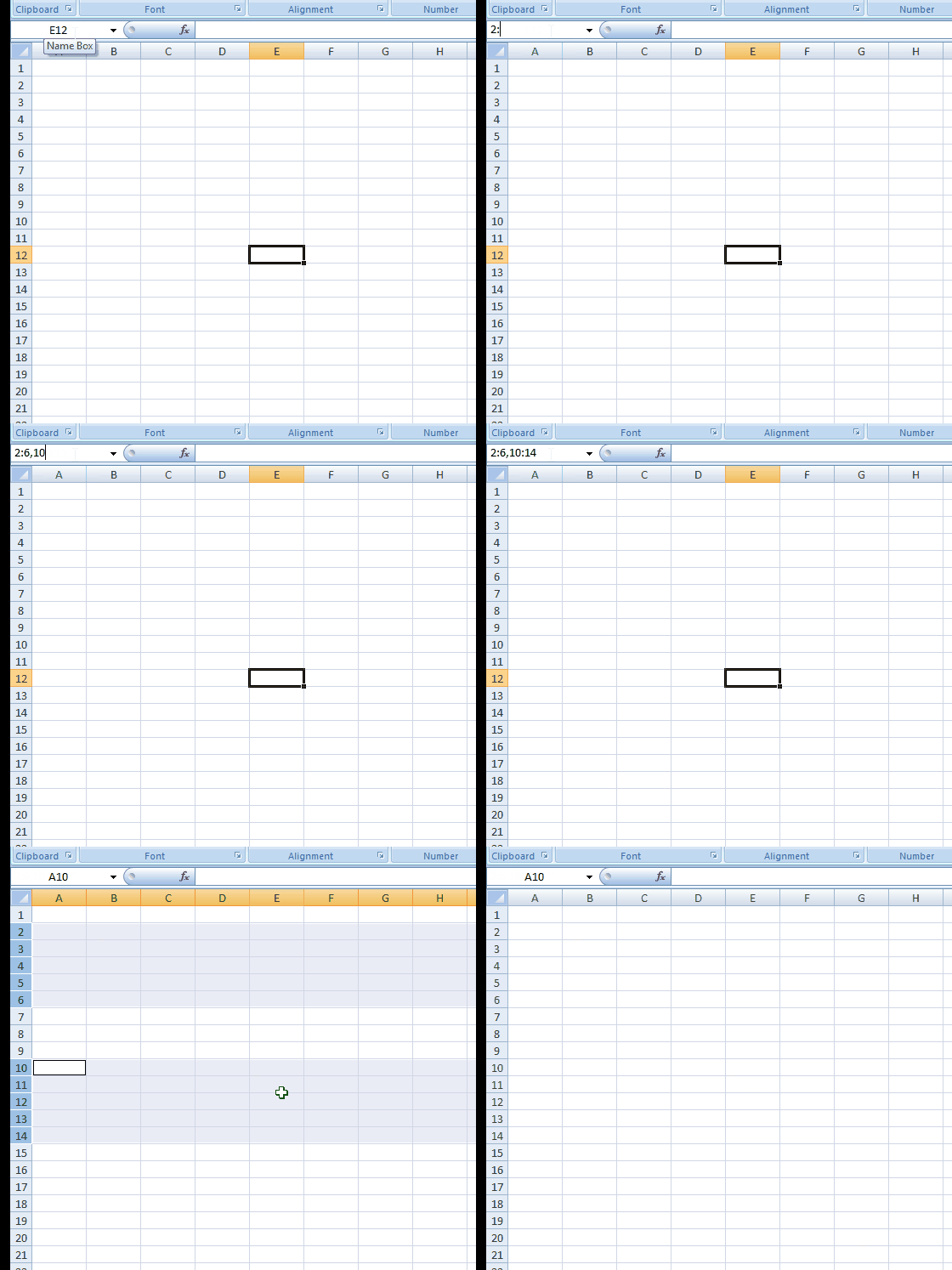
Previously, we saw (in point 5) a tip to select multiple particular range cells. In the same way, we can select multiple particular rows using the Name Box. Type 2:6,10:14 and hit enter. You see that rows 2 through 6 and 10 through 14 are selected.
Together select multiple particular entire row(s) and column(s)
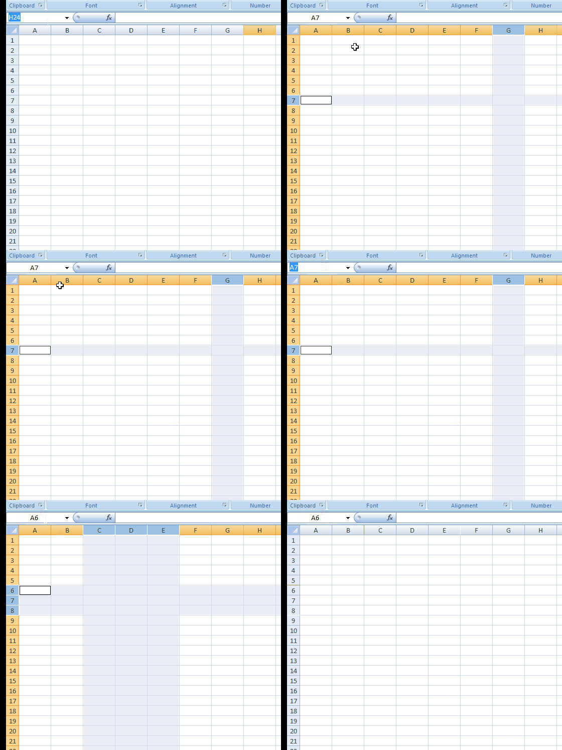
Type G:G,7:7 in the Name Box and hit enter. You see that entire column H and entire row 7 have been selected. In the same way, type C:E,6:8, and hit enter. You see columns C through E and 6 through 8 get selected together.
Select intersection region of specific row(s) and column(s)
This gives the same output as tip #2, but this time it identifies the region based on the intersection of rows and columns you mention in the Name Box. For example, we use the same values mentioned in tip #2. Type C:E 8:13 in the Name Box and hit enter. You see that C8 to E13 will be selected. Identify the space between E and 8.
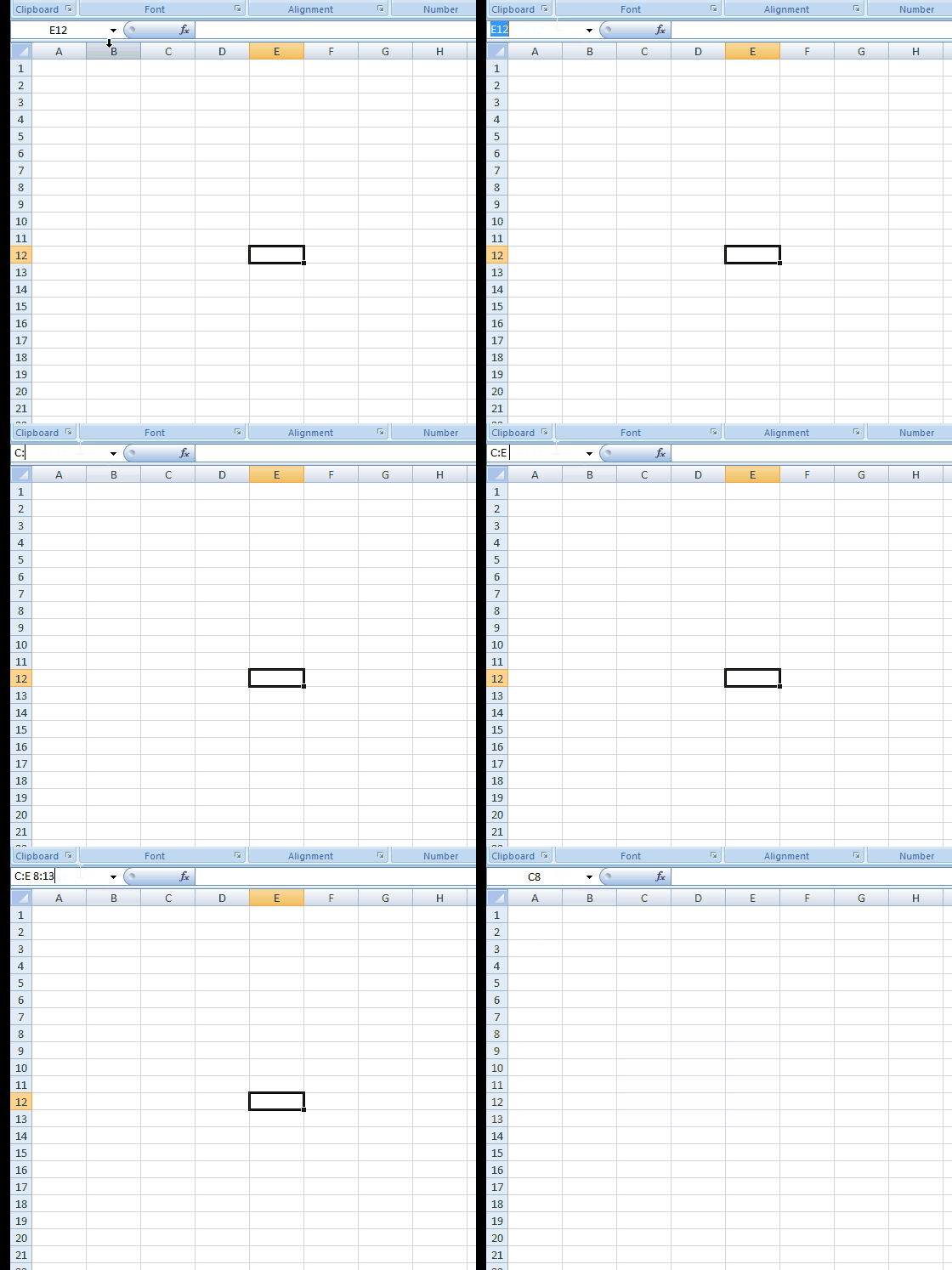
Here, the intersected area can be found by taking the first column in the mentioned range ‘C’ and the first row in the mentioned range ‘8’, and you get the first cell ‘C8’ of the intersection area. You can find the other cell value of the intersection area.
Tip to select the entire worksheet
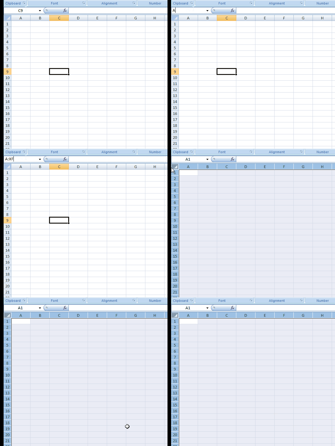
Type A:XFD in the Name Box and enter to see that the entire worksheet will be selected.
Add another selected region to the already selected region
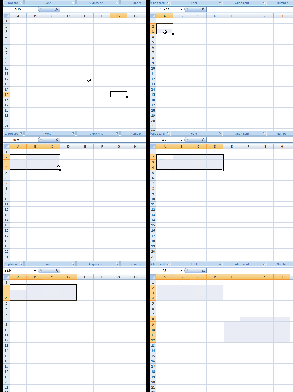
Select some region, say A2:D4 in the worksheet, and now type E8:H12 in the Name Box. Now, press and hold the Ctrl key on the keyboard and hit enter. You see, two ranges were selected A2 through D4 and E8 through H12. Try Shift and see the fun!
Select the entire column and a row of an active cell
Select any cell on the worksheet, type ‘C’ in the Name Box, and hit enter. You see that the entire column of that active cell gets selected. If you want to select the entire row of the active cell, then type ‘R’ in the Name Box and hit enter. This is one of the best ways to say the use of Name Box in Excel, isn’t it?
Get back to the active cell by collapsing the selected range
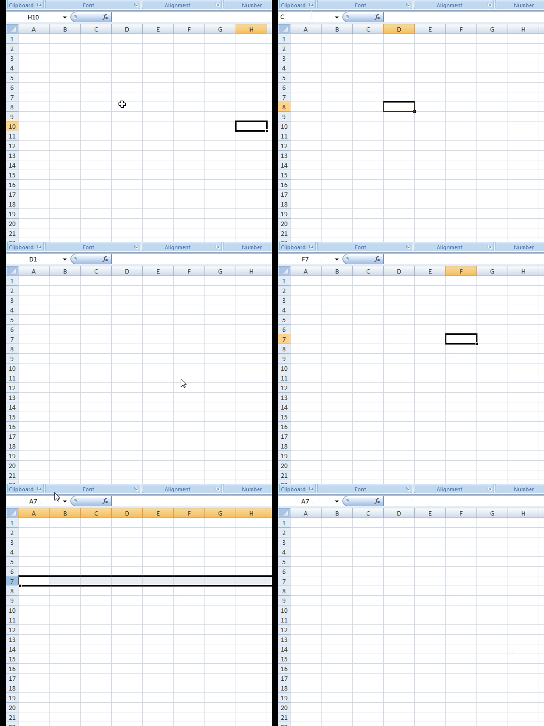
Select a range on the worksheet and type ‘RC’ in the Name Box. Hit enter, and you see that you get back to the active cell and the selection has collapsed.
Assign a name to the selected range
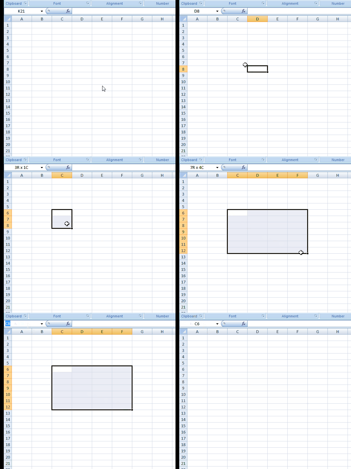
This tip shows you the use of Name Box in Excel. You can give a specific name to the selected range. Select a range on the worksheet and give the name in the Name Box, and hit enter. You can use this name in place of the selected range in any formula. This makes our task easier in such case.
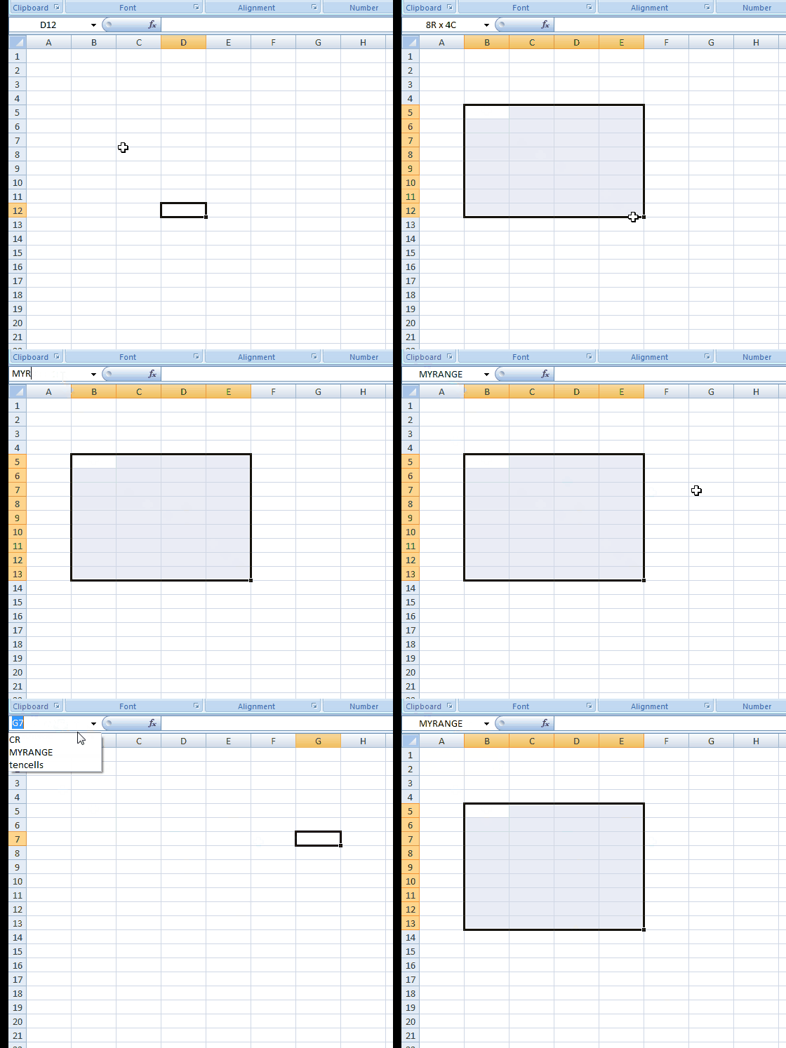
Later, if you want to select the same range, you can select the name from the Name Box. Remember that name should not have any spaces in it.
These are some tips and tricks for using Name Box in Excel best. I hope every tip will be useful to some or the other to make your task simpler. Try a few more with the help of these examples, and let us know. If you want to add anything to this, please do share it with us through comments.
Now see how to:
What is the shortcut to Name a cell in Excel?
When naming a cell or range in Excel, use the shortcut key Ctrl + F3 to open the Name Manager. In the Name Manager, you can create, edit, and delete any Excel names. Once a name is created, you can use the shortcut key F3 to insert any name into a cell.
Leave a Reply