Microsoft Excel has several accounting functions that help accountants work with large data sets easily and perform calculations of different types efficiently. Here, we will discuss some useful accounting Excel functions you can use to monitor, analyze, report, execute, and predict financial transactions.
Useful Excel Accounting Functions you should know
Here are the top useful accounting functions that accountants, aspiring accountants, and general users can use in Microsoft Excel for accurate and efficient calculations:
- SUMIF/SUMIFS/AVERAGEIFS/COUNTIFS
- SUMPRODUCT
- VLOOKUP
- TRIM
- AGGREGATE
- EOMONTH
- EDATE
- LET
- MATCH
- INDEX
- UNIQUE
- RATE
- FV
- PV
- PMT
- MIRR, IRR, ACCRINT
- DB, DDB
1] SUMIF/SUMIFS/AVERAGEIFS/COUNTIFS
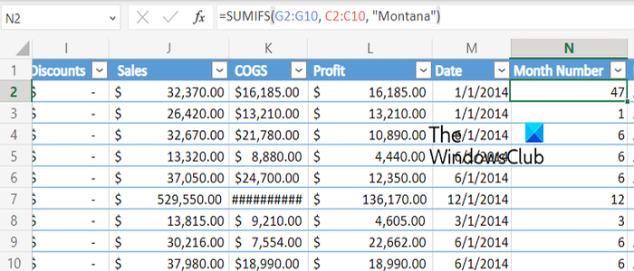
SUMIF, SUMIFS, AVERAGEIFS, and COUNTIFS are commonly used accounting functions in Microsoft Excel. These formulas are used to calculate cell values based on the criteria you have described or specified.
The SUMIF function in Excel is used to add all the cell values and return the results on the basis of one criterion. On the other hand, the SUMIFS formula enables you to sum up all cell values on the basis of more than one criterion.
AVERAGEIFS lets you calculate the average of cells on the basis of multiple defined criteria. Similarly, if you want to count the number of times all your specified criteria are met, you can use the COUNTIFS function in your Excel worksheet.
Here are the examples of each of these formulas:
- =SUMIF(A2:A25,”>10″) to add values that are larger than 5.
- =SUMIFS(A2:A9, B2:B9, “=B*”, C2:C9, “Komal”) to add the number of products beginning with B and sold by Komal.
- =AVERAGEIFS(B2:B5, B2:B5, “>70”, B2:B5, “<90”)
- =COUNTIFS(B2:B5,”=Yes”,C2:C5,”=Yes”)
2] SUMPRODUCT
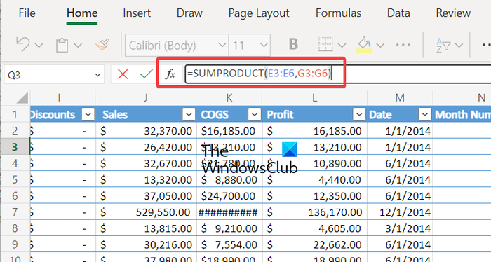
SUMPRODUCT is another widely used Excel function. It is used to add up values of multiple ranges or arrays.
For example, if you use the =SUMPRODUCT(C2:C5,D2:D5) formula, it will multiply values in the C column to the corresponding cells in the D column and then sum up all the calculated products. The multiplication is done by default. However, you can also use it for addition, subtraction, and division.
3] VLOOKUP
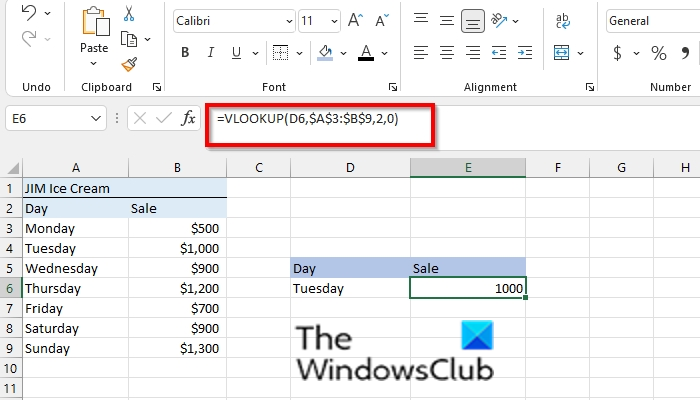
Well, accountants must be familiar with the VLOOKUP formula in Excel. It is one of the prominent formulas in Excel that enables you to search for specific things in a table or range. Let’s say you want to look up an order name based on the order number, you need to use VLOOKUP. It searches values in columns. If you want to look up values in horizontal data, HLOOKUP, INDEX and MATCH, or XLOOKUP can be used.
The syntax for the VLOOKUP formula in Excel is as follows:
VLOOKUP(lookup_value, table_array, col_index_num, [range_lookup])
Here is a full guide to using the VLOOKUP function in Excel.
4] TRIM
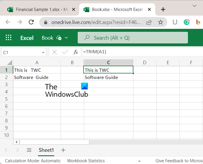
TRIM, as the name suggests, is an Excel formula that you can use to trim or remove extra or redundant space in the text. Extra spaces are likely to cause errors with used formulas and return incorrect values or errors. Hence, to avoid any errors in using formulas, we use the TRIM function.
Its syntax is very easy. Suppose, you want to clear extra spaces in B1 cell, you will use the below formula:
=TRIM(B1)
In case you want to delete spaces, line breaks, and other unneeded characters from cell C1, you can enter the below formula:
=TRIM(CLEAN(A1))
There are more syntaxes used for this formula that vary as per your requirement.
Read: How to use the ISNUMBER function in Excel?
5] AGGREGATE
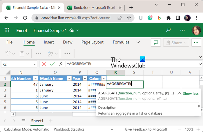
The next Excel accounting formula that we would like to list is the AGGREGATE function. It is a built-in function in Excel that is used to apply functions like AVERAGE, SUM, COUNT, etc., to a list or database while ignoring hidden rows and error values.
The syntaxes to apply this function in your Excel worksheet are as follows:
AGGREGATE(function_num, options, ref1, [ref2], …)
AGGREGATE(function_num, options, array, [k])
6] EOMONTH
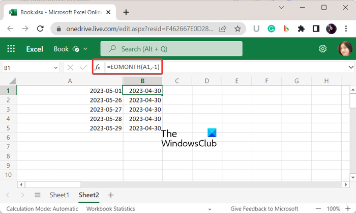
EOMONTH is another important Excel accounting formula that returns the maturity dates or due dates falling on the last day of the month. Its syntax is very simple. It is as follows:
EOMONTH(start_date, months)
In the above formula, you need to mention the starting date and the number of months before or after the starting date. If you enter a negative value for the month, it will produce the past date.
For example:
=EOMONTH(A2,-3)
If the starting date is 1-Jan-23, the above formula will calculate 31/10/2022.
See: Microsoft Excel shortcut keys and their functions.
7] EDATE
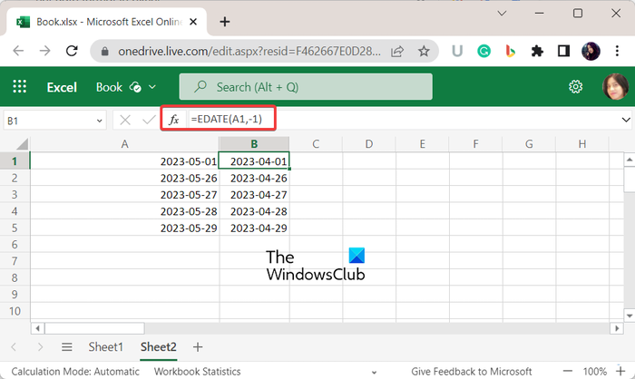
EDATE is a date and time Excel function that calculates due dates falling on the same day of the month as the issue date. Its syntax is similar to the EMONTH function.
EDATE(start_date, months)
For example:
=EDATE(B2,-1)
The above formula will calculate the date one month before the date mentioned in the B2 cell.
8] LET
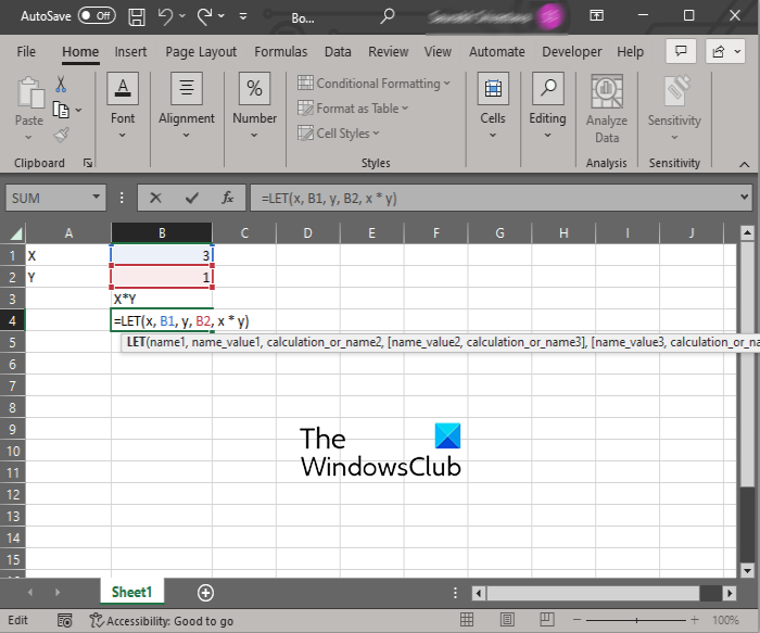
Another Excel accounting formula is LET. This function enables users to assign names to the results of calculations, and you can also define variables inside a formula using it. This function is used to make a formula look clearer and run faster.
Syntax of LET function is:
=LET(name1, name_value1, calculation_or_name2, [name_value2, calculation_or_name3...])
The primary reason for using the LET function is to simplify the formulas used in your Excel worksheet. It is also easier to maintain and update and calculates faster.
This function can be used in Excel 365, Excel Online, and Excel 2021 versions.
Read: How to create Custom Excel Functions using VBA?
9] MATCH
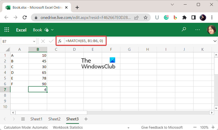
MATCH is an Excel accounting function that is used for searching the exact position of an item within a given range of cells. The syntax of the MATCH function is as follows:
MATCH(lookup_value, lookup_array, [match_type])
Now, suppose, you have 35 and 65 values in A1 and A2 cells and you want to know the position of 65, you can use the below formula:
=MATCH(C,A1:A2,0)
The above formula will return “2” since 65 is present in the A2 cell. Similarly, you can find out the position of any item or value within a provided range.
10] INDEX
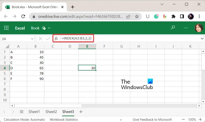
The Excel function INDEX is used for calculating a value or the reference to a value within a specified table or range in a dataset. You can use it using the below syntax:
INDEX(array, row_num, [column_num])
INDEX(reference, row_num, [column_num], [area_num])
11] UNIQUE
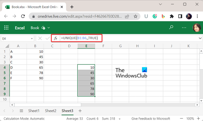
As the name suggests, UNIQUE is an Excel function that returns that values that are unique in a specified range of cells. Here is its syntax:
=UNIQUE(array,[by_col],[exactly_once])
The exactly_once argument can be set to True to calculate the unique values in a list or range.
For example:
=UNIQUE(A1:A16,,TRUE)
It will return all unique values from A1 to A16 cells.
Read: How to use the MINVERSE and MMULT functions in Excel?
12] RATE
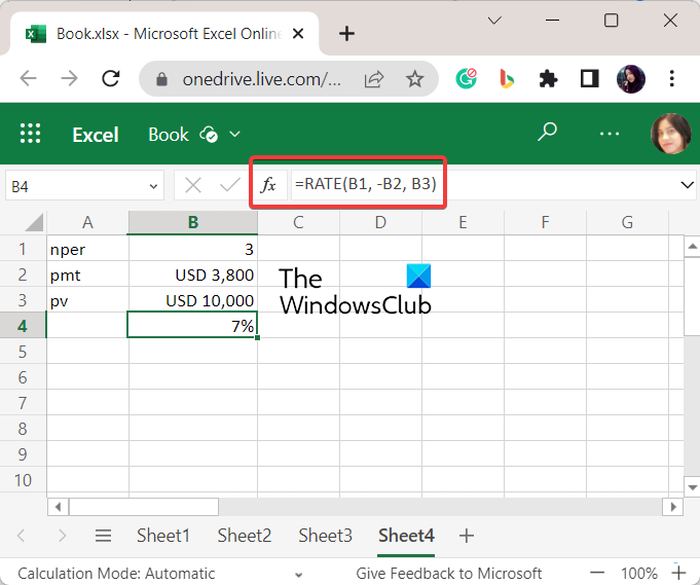
The RATE function in Microsoft Excel is used to calculate the interest rate per period of an annuity. The syntax for using this function is as below:
RATE(nper, pmt, pv, [fv], [type], [guess])
In the above syntax, nper, pmt, and pv arguments are required. While the fv, type, and guess arguments are optional.
13] FV
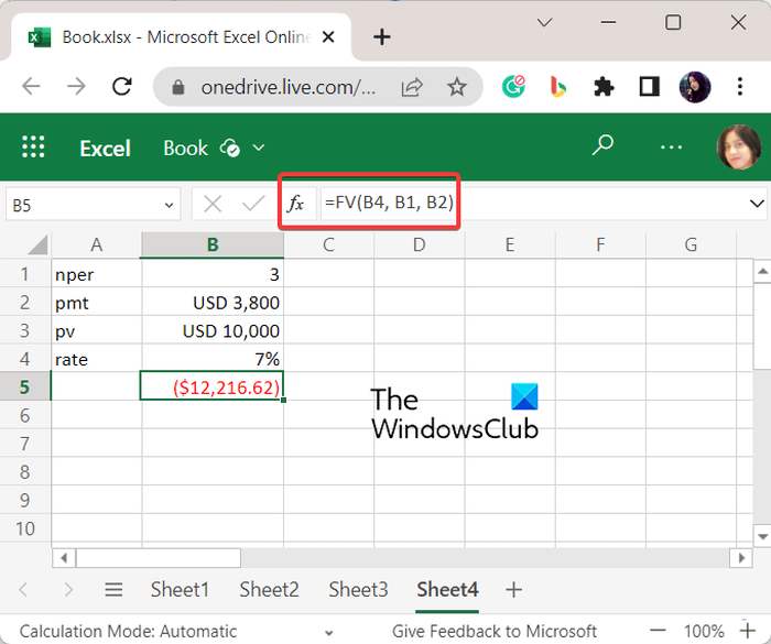
FV is a financial Excel function that can be used to calculate the future value of an investment on the basis of a constant interest rate. It is a very useful accounting function that is used by accountants.
Syntax:
FV(rate,nper,pmt,[pv],[type])
In the above syntax, the rate is the interest rate per period, nper is the number of payment periods, and pmt is the payment made each period. These are required arguments. On the other hand, pv is the present value which is optional. The type argument is also optional and it indicates when is the payment due.
You can use this function to calculate the future value of your investments or savings accounts.
Read: How to use the IMCOS function in Microsoft Excel?
14] PV
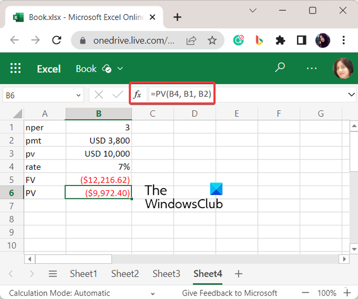
PV is one more accounting Excel formula on this list. If you want to calculate the present value of a loan or an investment, you can use this formula. This function can be used using the following syntax:
=PV(rate, nper, pmt, [fv], [type])
The arguments used in this function are the same as the above-listed FV function. Just fv is used for the final value.
15] PMT
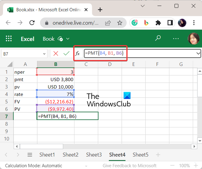
PMT stands for Payment. This Excel function can be used to calculate the monthly loan payment on the basis of the constant interest rate, the number of periods, and the total loan amount. The syntax for this formula is:
PMT(rate, nper, pv, [fv], [type])
The arguments used in this function are the same as described for the FV and PV functions.
16] MIRR, IRR, ACCRINT
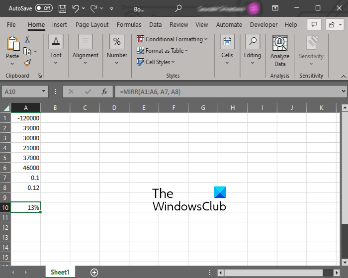
MIRR stands for modified internal rate of return. It is used to compute the cash flows of a company. To use this Excel function, the syntax is:
MIRR(cash_flows, finance_rate, reinvest_rate)
IRR is another accounting function in Microsoft Excel that is used for estimating the internal rate of return for cash flows. The syntax for this function is:
IRR(values, guess)
ACCRINT is one more Excel function for accountants that enables them to compute the accrued interest over a time period for security.
ACCRINT(id, fd, sd, rate, par, freq, basis, calc)
In the above syntax, id is the issue date, fd is the first interest date, sd is the settlement date, rate is the interest rate, par is the security’s par or face value, and freq is the number of payments per year. basis and calc are optional parameter controls.
17] DB, DDB
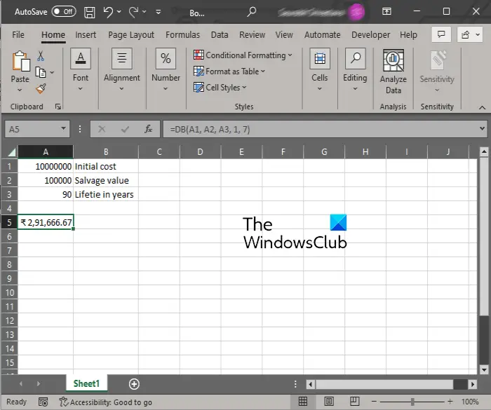
DB function is used to estimate the depreciation of an asset using the Fixed Declining Balance Method. On the other hand, DDB is used for computing the depreciation of an asset for a given time period using the double-declining balance method. Here are the syntaxes used for these two functions:
=DB(cost, salvage, life, period, [month])
=DDB( cost, salvage, life, period, [factor] )
Hope this post helps you learn some useful accounting functions in Microsoft Excel.
Now read: 10 Text functions in Excel with examples.
What are 5 main functions used in Excel?
The five widely used functions in Excel are SUM, AVERAGE, COUNT, SUBTOTAL, and CONCATENATE. These functions are used by most users. However, the top functions can vary on the basis of your main purpose. If you want to use functions for accounting purposes, SUMPRODUCT, VLOOKUP, TRIM, AGGREGATE, and SUMIFS are some prominent Excel functions.
What is the one function in Excel that every accountant should be familiar with?
There are a lot of functions in Microsoft Excel that an accountant must know of. Some of these functions include MIRR, IRR, ACCRINT, VLOOKUP, FV, PV, PMT, etc. We have shared a list of other useful accounting functions that you can check out below.