In spite of having several spreadsheet tools and other similar applications, we still prefer to work along with Microsoft Excel itself. This is because this spreadsheet program makes your job pretty handy if you know the way to use it. Whether you are a small businessman or working in a corporate office, Excel worksheet has now become a quite helpful and essential resource for daily users.
This application is mainly used for recording and manipulating numerical data for various purposes. Because of its straightforward functions and easy-to-use features, it has been always the primary means of every corporate user. In this guide, there are 10 major helpful Excel tips and tricks that one must know.
Microsoft Excel Tips and Tricks
In this post we will cover the following Excel Tips and Tricks, which we think are the most useful ones:
- Select all cells at once
- Autofit Column width
- Transpose columns and rows
- Use Filter Command to Hide Unwanted Data
- Remove Duplicate Entry
- Remove the Blank Records
- Insert Blank Rows into Record
- Copy Data to Another Sheet Automatically
- Take Screenshot using Excel Camera
- Link the cells to your email address
Let us start and know each one in detail.
1] Select all cells at once
Sometimes you might need to make some massive changes to your Excel worksheet. In such a case, you can select all the cells in your worksheet using the square box that is available in the extreme top-left corner of the spreadsheet.
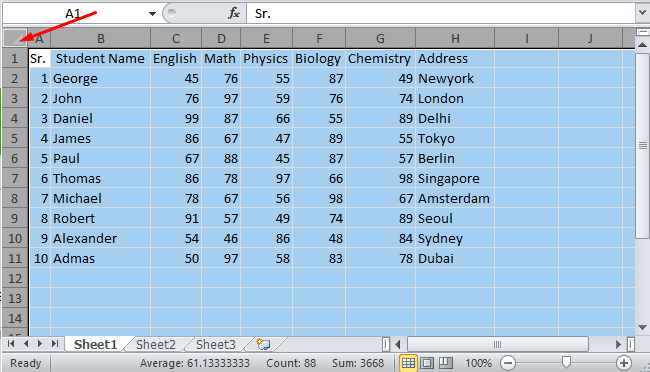
When you select the square box, it highlights all the cells in the worksheet even the empty cells as well. As an alternative, you can also use the Ctrl+A keyboard shortcut to select all the cells on the worksheet.
Read: Microsoft Excel Tutorial for Beginners
2] Autofit Column width
While working on the MS Excel with a large amount of data record, often it becomes complicated to resize each column cells according to its text. In order to resize the columns in an easy way, you can use the AutoFit column width feature that is an inbuilt feature in Excel.
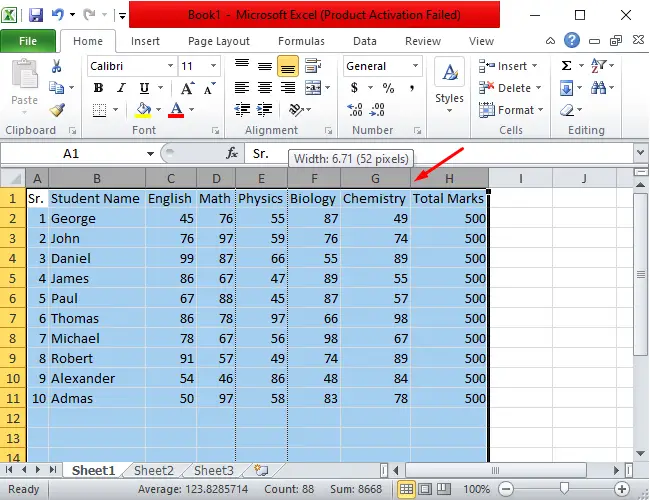
You need only move your mouse pointer to the boundary of the column you want to autofit and then double-click on it. If you have to adjust all the columns, then select them all and double-click on the boundary of any column.
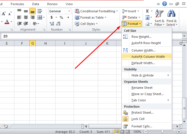
Alternatively, you can also resize the column width by using the Autofit Column width option. To do this, select the column you want to adjust and then navigate to the Menu bar > Home tab. In the Cells section, click on the Format option and then select Autofit Columns Width from the drop-down menu.
Read: List of best free Excel Add-ins you should be using
3] Transpose columns and rows
Some people create Excel spreadsheets where the main fields go across horizontally in a row. Others put the data vertically. Sometimes these preferences lead to a scenario where you want to transpose Excel data. Transpose is an Excel function that allows you to switch Excel columns to rows without retyping the data.
The Transpose function is a great feature in MS Excel spreadsheets. It is very helpful when you need to switch the data columns from horizontal to vertical without retyping the data.
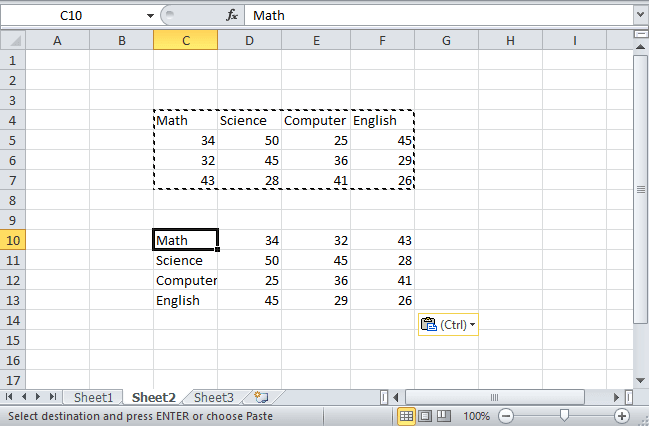
In the above picture, the data are arranged in tabular form, with the figures of the subjects shown vertically. Rearranging the data horizontally manually would be quite difficult, but with the help of the transpose function, you can do it in a couple of seconds.
So, you first need to select the data from the table and copy it. Now, place your mouse pointer where you have to transpose the data, right-click, and select the Paste Special option from the context menu. When the Paste Special window opens, check the Transpose function and click on the OK button.
Read: Top 15 Financial functions in Microsoft Excel
4] Use Filter Command to Hide Unwanted Data
Excel filter function allows you to hide the unwanted data and to display only certain important data in the spreadsheet. This feature lets you easily filter the names, dates, and numbers from the huge dataset or table. However, it doesn’t remove or modify the original data. It becomes very useful when focusing only on some special kind of information.
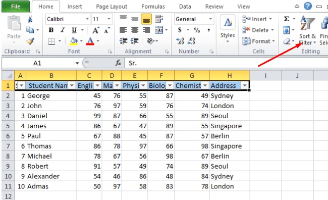
In the above dataset, you can see there is a list of students whose marks and addresses are different. The list can be even larger. So, if you need to filter any specified data, then it can be quite difficult.
You can use the filter command to make it easy. To do so, select the table header and then navigate to the Editing section. In the corresponding section, select Sort & Filter and then choose the Filter tool.
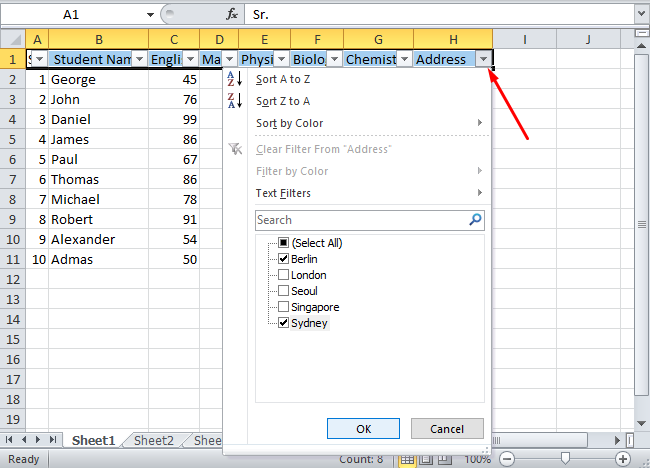
Click on the down-arrow option that comes to appear near the header of each column. It allows you to sort your data in alphabetical order or to arrange the numbers by smallest to largest. Furthermore, you can use the text filter to filter the data as per your requirement.
5] Remove Duplicate Entry
It is quite easy to locate and remove duplicate entries in a spreadsheet with a small set of data. But if it has to be done with a large dataset with hundreds of columns and rows, then it would be indeed a challenging task.
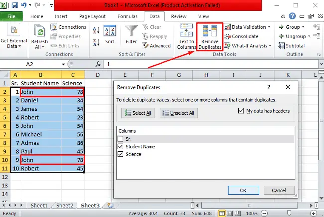
In the above table, there are ten records in which two entries are totally similar and a common name has been used in three rows. So, to find out the duplicate entries, you need to select the table. After that, navigate to the Data menu, select the Data Tools category, and then click Remove Duplicates.
In the dialog box, mark the checkbox near the My data has headers. And, under the columns section, remove the mark of the serial number as it is different for each entry. Finally, click on the OK button and you will see the duplicate entry gets removed from the table.
6] Remove the Blank Records
Sometimes you might have noticed the blank cells or rows in your spreadsheet that are mostly undesirable. Users commonly do a right-click on the specified row and delete them one by one. But what will you do if their numbers are in the hundreds? Deleting them one by one would be a tedious job in that situation.
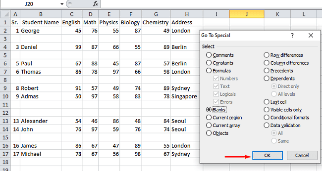
Therefore, in order to delete them in one go, press Ctrl+G shortcut key and when the Go To dialog box comes to appear, select the Special button. On the following page, mark the Blanks radio button and click on the OK button. You will notice that all the blank cells get selected.

Now, press the Ctrl+minus button. When a pop-up menu appears, select Shift cells up and click on the OK button. You will see, all the blanks cells get removed and the dataset also arranged suitably.
7] Insert Blank Rows into Record
As I mentioned, blank rows are mostly undesirable, but sometimes they work as well. So, if you need to insert them, you can right-click on the specified row and add them one by one, as I stated while removing blank rows.
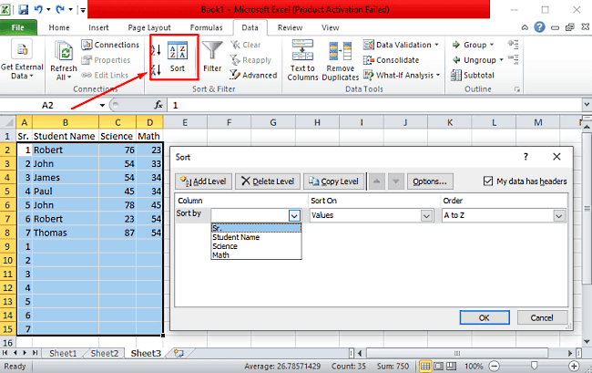
So, to insert the blank rows in each separate record, make a series of the mentioned serial number. After that, select all the data set and then click on the Sort tool available on the Data tab.
In the following dialog box, click on the Sort by drop-down menu and arrange the items by serial number.
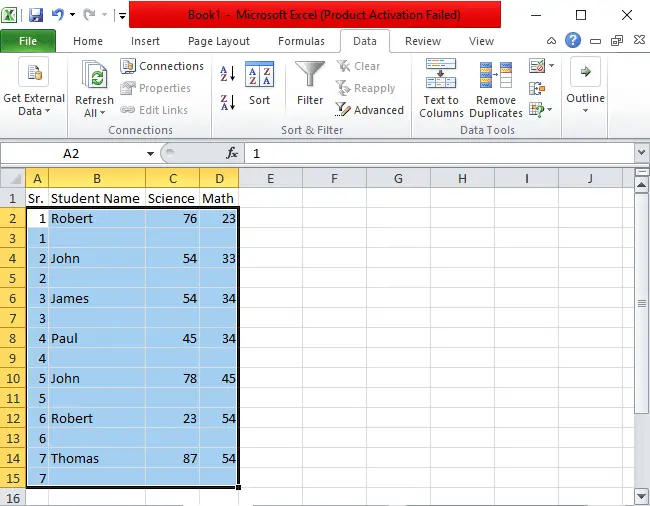
Clicking on the OK button, it will insert a blank row between each separate row.
8] Copy Data to Another Sheet Automatically
Sometimes it happens that you need to use the data in another sheet, which you entered in the first sheet. To do so, you commonly use the traditional copy and paste method. But, when you need to change some data in one sheet, then it has to be changed on the other sheet as well. It becomes a bit complicated when you have to change the same data on both sheets one by one.
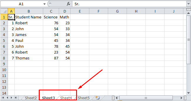
In excel, there is an option that automatically copies the data of the first sheet into other sheets in a real-time process. However, for copying the data automatically to other sheets, you need to first make a connection between them.
To do so, go to the status bar of the first sheet. After that, keep pressing the Ctrl key and click those sheets on which you have to copy the data automatically. That’s it.
Now whatever data you enter on the first sheet, it automatically gets copied on the other sheets.
9] Take Screenshot using Excel Camera
It has always been said that “A picture is worth a thousand words”. Accordingly, sometimes you may need to add a screenshot within your Excel worksheet so that you could explain the things in a better way.
However, you don’t need to use a third-party application to capture a screenshot. Excel has an inbuilt camera command that allows you to take a screenshot with a single click.
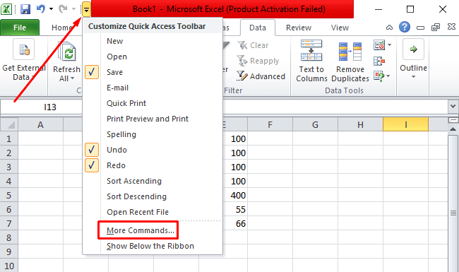
To use this feature, you first have to enable the camera command. So, all you need to navigate to the quick access toolbar and click on the Customize Quick Access Toolbar. After that, click on the drop-down menu of Choose commands from > All commands > Camera. Now, select the Add button and hit OK.
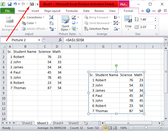
After following the above procedure, you will notice a Camera icon has been added to the quick access toolbar. Select the cells or data for which you need an image. Then, click on the Camera icon and anywhere on the worksheet. You can also drag and resize the image to adjust it according to your requirements.
10] Link the cells to your email address
In the excel worksheet, you can easily create a hyperlink to your Gmail address.
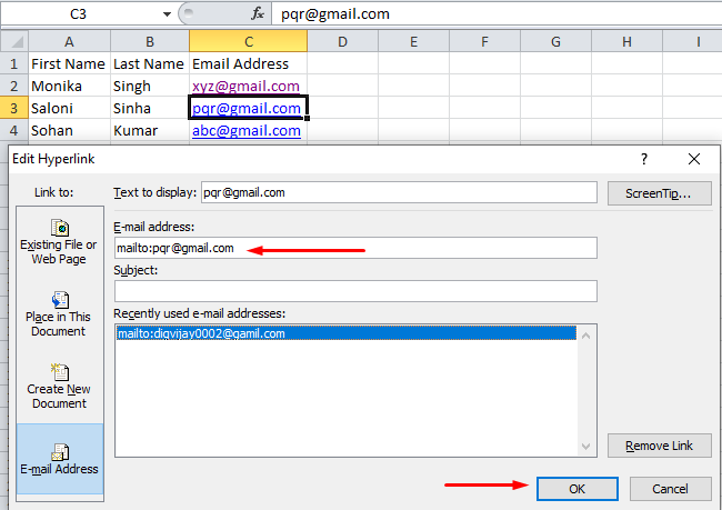
To do so, you must select the cell where you want to insert the link. After that, press Ctrl+K shortcut. When the dialog box prompts on the screen, select the E-mail Address from the left pane. Add your email address and then hit the OK button.
That’s it. I hope these tips and tricks will help you use Excel worksheets on your computer.
Now read: Advanced Microsoft Excel Tips and Tricks for Windows users.
Leave a Reply