This post explains what is IFERROR function and how to use the function in Microsoft Excel. The IFERROR function was introduced in Excel as a logical function to handle errors that may occur within formulas or calculations in Excel. It is now available in all the versions of Excel, including Excel for Microsoft 365.

The IFERROR function can handle the following errors in Excel: #N/A, #DIV/0!, #NULL!, #NAME?, #NUM!, #VALUE!, and #REF! If you want to know how to use the IFERROR function to suppress the error when your argument refers to one of these error values, continue reading this post.
What is IFERROR function in Excel?
When a formula evaluates to incorrect results, an error code appears in the cell in Excel. For example, if you apply a formula to calculate the sum of values from 2 cells but the 1st cell contains a text value, the formula returns the #VALUE! error. Similarly, if you apply a formula to divide something by 0 or an empty cell value, Excel returns the #DIV/0! error.
Not every user is familiar with these error codes and if you’re collaborating on an Excel document or going to share it with your colleagues or readers, you might want to replace the error code with something more meaningful and sensible. Here’s where the IFERROR funtion comes into play. It replaces the error code with a custom text message or a logical value if the formula evaluates to an error, and otherwise, returns the results of the formula.
The IFERROR function has the following syntax:
IFERROR(value, value_if_error)
Where,
- value refers to the formula or expression that needs to be evaluated for an error. It could be a value or a cell reference.
- value_if_error refers to the output to be returned if the formula evaluates to an error. It could be a text message, a numeric value, an empty string, etc.
How to use the IFERROR function?
Let us understand how to use the IFERROR function in Excel with the help of an example.

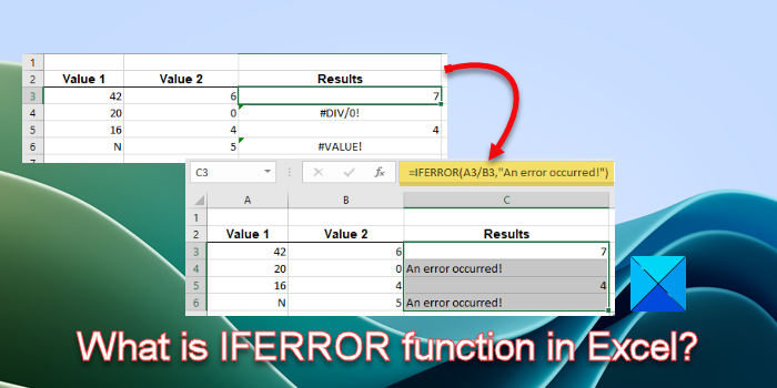
Suppose we have a worksheet wherein we have some values listed in two different columns, as shown in the above image. The idea is to divide the values of Column A by the values of Column B. So we’ll place the cursor in cell C3 and type the following formula:
=A3/B3
Upon pressing the Enter key, the formula evaluates to ‘7’, which is what we get after dividing 42 by 6.

Next, we will take the cursor to the bottom-right corner of cell C3, and as it converts to a plus (+) symbol, we click and drag the cursor downwards till cell C6, and then release the cursor. This action will copy the formula entered in cell C3 to cells C4, C5, and C6. For each pair of values (A4/B4, A5/B5, A6/B6), the formula evaluates to the following results:

As you can see, the formulas in cell C4 and cell C6 evaluate to a #DIV/0! error and a #VALUE! error. To replace these error codes with a pre-defined error message, we can use the IFERROR function as follows:
=IFERROR(A3/B3,"An error occurred!")
After enclosing the Division formula within the IFERROR function, the following results will be obtained:

So basically, if the formula passed in the first argument of the IFERROR function returns an error value, the IFERROR function returns the text passed in its second argument in place of the error.
Similarly, we can apply the IFERROR function to hide all major error codes in Excel behind a user-defined value.
Tip: You can use IFERROR with VLOOKUP to elegantly trap and handle errors (or tell users the value they’re looking for is not in the dataset).
That’s it! I hope this helps.
Also Read: How to use the PROPER function in Excel.
How do you enter an Iferror function?
Place your cursor in the cell that holds the existing formula. Then take your cursor to the formula bar and place it next to the equals to symbol (=). Type ‘iferror’ and press the Tab key to select IFERROR from the list of suggested Excel functions. Move your cursor to the right of the existing formula and enter a comma symbol. Now enter your custom text within double quotes and close the parenthesis of the IFERROR function. Press Enter to generate the results.
What is Iferror and if in Excel?
The IF function makes a logical comparison between two values. It returns TRUE if the condition is met; else, it returns FALSE. The IFERROR function allows users to handle errors in Excel formulas. If there is an error in the formula, it returns a pre-defined value; otherwise, it returns the results of the formula.
Read Next: How to use the COUNTA function in Excel.